
DotPlots for comparing genomes
One of the primary comparative analyses that can be done once you have the genome is by visualizing the synteny with closely related species. Many characteristics for the genome can be easily highlighted with a good dotplot. Structural variations like inversion, deletion, duplication and insertions can be identified from these dotplots.
You will need two genomes for generating dotplots. A higher quality, preferably at chromosome level “reference” genome (also referred as target genome) and your genome (scaffold or contigs are okay, but chromosomes would be ideal), which is referred as query genome. We will run this tutorial using maize genomes, but can be easily applied on any other genome as well.
Data
Download the data from Grameme and MaizeGDB
1
2
3
4
5
6
7
# B73 version 4.0 (Target)
wget ftp://ftp.gramene.org/pub/gramene/release-61/fasta/zea_mays/dna/Zea_mays.B73_RefGen_v4.dna.toplevel.fa.gz
# Genome of interest (Query)
wget https://ftp.maizegdb.org/MaizeGDB/FTP/Zm-CML247-REFERENCE-PANZEA-1.1/Zm-CML247-REFERENCE-PANZEA-1.1.fa.gz
# maize custom TE libraries
wget https://de.cyverse.org/dl/d/66ACA7F8-A367-4C48-9D63-828788F4F559/maizeTE10102014.RMname.nogene
gunzip *.gz
Overview
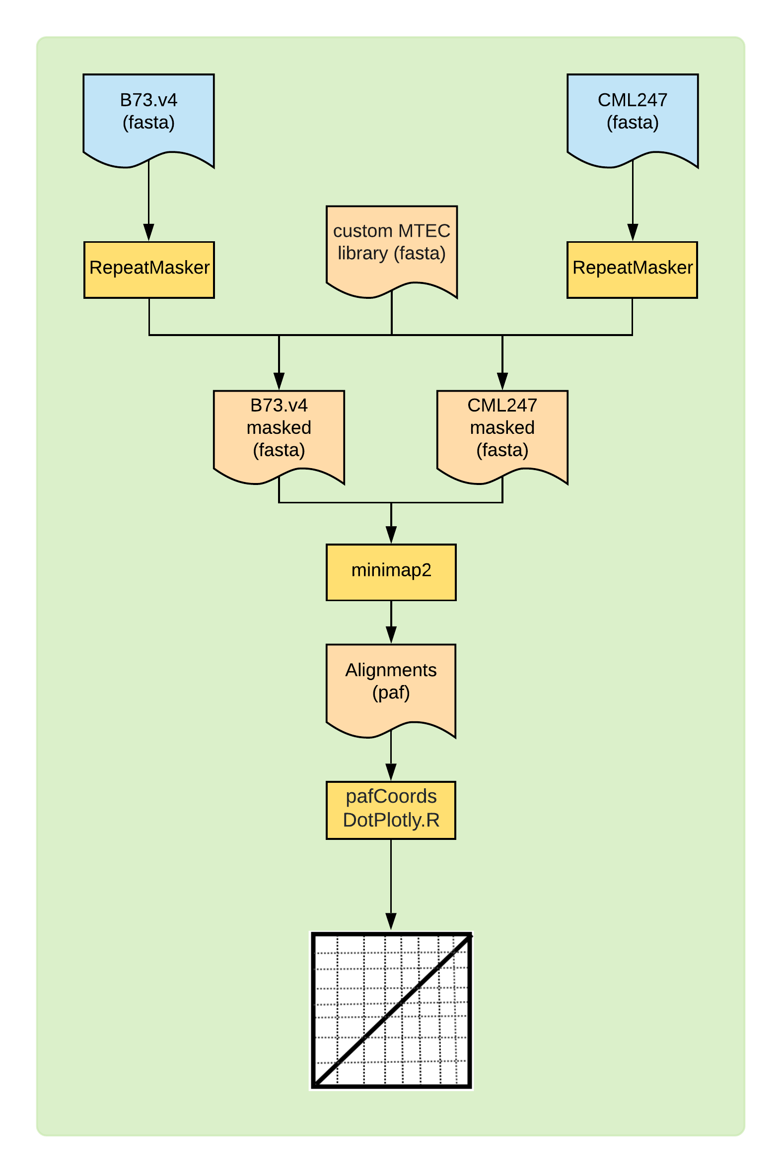
Figure 1: Overview of the DotPlot construction method
Organization
1
2
3
4
5
6
7
8
9
10
11
SyntenyTutorial
├── 1_data
│   ├── Zea_mays.B73_RefGen_v4.dna.toplevel.fa
│   └── Zm-CML247-REFERENCE-PANZEA-1.1.fa
├── 2_repeatmasking
│   ├── runRepeatMasker.sh
│   └── maizeTE10102014.RMname.nogene
├── 3_minimap
│   └── runMinimap.sh
└── 4_paf-processing
    └── pafCoordsDotPlotly.R
Programs needed
Following programs are needed for this tutorial. Most of them can be installed via Conda environment, but some of them can be directly cloned from GitHub:
1. Repeatmask the genomes
For masking the maize genomes, it is essential to have an accurate, custom TE library. Using a generic repeat database will mask the genic regions and other potentially non-repetitive portions of the genome, leading to inaccurate downstream analyses.
Ou Shujun, from Hufford Lab, here at ISU created a new maize repeat library, using The Extensive de novo TE Annotator (EDTA). This is the Maize TE Consortium (MTEC) curated TE library created in 2014/10/10. The original sequence names were converted to fit the naming scheme of RepeatMasker, so that TEs could be parsed into class, super-families, and families. A TE-free whole-genome CDS dataset derived from the B73v4 annotation was used to clean any potential genic sequences in this MTEC library. TE sequences containing more than 1000 bp or 30% of genic sequences were discarded entirely, otherwise genic sequences were removed and the remaining sequences were joined. Cleaned TE sequences shorter than 80 bp were also discarded. As terminal structure of TEs is the key for their identification, any TE sequences with the beginning or ending 20 bp masked by CDS sequences were determined false positives and removed. Overall, a total of 1,359 sequences were remained from the original 1,546 sequences.
Setup
1
2
3
cd 2_repeatmasking
ln -s ../1_data/Zea_mays.B73_RefGen_v4.dna.toplevel.fa
ln -s ../1_data/Zm-CML247-REFERENCE-PANZEA-1.1.fa
Script runRepeatMasker.sh
1
2
3
4
5
6
7
8
9
10
11
12
#!/bin/bash
conda activate repeatmasker
lib="maizeTE10102014.RMname.nogene"
genome=$1
RepeatMasker \
  -e ncbi \
  -pa 36 \
  -q \
  -lib ${lib} \
  -nocut \
  -gff \
  ${genome}
Generate commands and submit:
1
2
3
4
5
6
7
for fasta in *.fa; do
  echo "./runRepeatMasker.sh $fasta"
done > repmask.cmds
makeSLURMs.py 1 repmask.cmds
for sub in repmask_*sub; do
  sbatch $sub;
done
Once complete, you will have following output files:
For B73.V4:
1
2
3
4
5
6
Zea_mays.B73_RefGen_v4.dna.toplevel.fa.out
Zea_mays.B73_RefGen_v4.dna.toplevel.fa.masked
Zea_mays.B73_RefGen_v4.dna.toplevel.fa.tbl
Zea_mays.B73_RefGen_v4.dna.toplevel.fa.ori.out
Zea_mays.B73_RefGen_v4.dna.toplevel.fa.cat.gz
Zea_mays.B73_RefGen_v4.dna.toplevel.fa.gff
Here, the <name>.fa.gff provides a GFF file for masked regions, that can be visualized in IGV and the <name>.fa.masked provides you a masked genome that is needed for our subsequent steps.
2. MiniMap2 to align genomes
Although there are many programs to align the genomes, MiniMap2 does the job really well at lightning speed. The repeatmasked genomes can be aligned in less than 10 minutes, running on a cluster with 16 CPUs, 128Gb RAM. Moreover, the preset options eliminates a guess work of what options that might or might not work for your specific condition. The aligner is also versatile and can use many different data inputs as well.
Setup:
1
2
3
cd 3_minimap
ln -s ../2_repeatmasking/Zea_mays.B73_RefGen_v4.dna.toplevel.fa.masked B73.v4-masked.fa
ln -s ../2_repeatmasking/Zm-CML247-REFERENCE-PANZEA-1.1.fa.masked CML247-masked.fa
Script runMinimap.sh
1
2
3
4
5
6
#!/bin/bash
query=$1
target="B73.v4-masked.fa"
outname="${query%.*}_${target%.*}_minimap2.paf"
module load minimap2
minimap2 -x asm5 -t 36 $target $query > ${outname}
Generate commands and submit:
1
2
3
echo "./runMinimap.sh CML247-masked.fa" > minimap.cmds
makeSLURMs.py 1 minimap.cmds
sbatch minimap_0.sub
The resulting file will be
1
CML247-masked_B73.v4-masked_minimap2.paf
Which is now ready to plot.
3. Dot plot
For Dot plot, we will use dotPlotly. There is a R Shiny app as well, but there is a limit on the file size that can plotted. Morover, if you upload a complex file like maize alignment, it will be very sluggish and interactive-ability will not be usable. So, we will download the script and run them locally to generate a static dotplot.
Setup:
1
2
cd 4_paf-processing
ln -s ../3_minimap/CML247-masked_B73.v4-masked_minimap2.paf
Download program
1
git clone https://github.com/tpoorten/dotPlotly.git
Run the script:
1
2
3
4
5
6
7
./dotPlotly/pafCoordsDotPlotly.R \
   -i CML247-masked_B73.v4-masked_minimap2.paf \
   -o CML247.plot \
   -m 2000 \
   -q 500000 \
   -k 10 \
   -s -t -l -p 12
The stdout:
1
2
3
4
5
6
7
8
9
10
11
12
13
14
15
16
17
18
19
20
PARAMETERS:
input (-i): CML247-masked_B73.v4-masked_minimap2.paf
output (-o): CML247.plot
minimum query aggregate alignment length (-q): 5e+05
minimum alignment length (-m): 2000
plot size (-p): 12
show horizontal lines (-l): TRUE
number of reference chromosomes to keep (-k): 10
show % identity (-s): TRUE
show % identity for on-target alignments only (-t): TRUE
produce interactive plot (-x): TRUE
reference IDs to keep (-r):

Number of alignments: 186189
Number of query sequences: 608

After filtering... Number of alignments: 64210
After filtering... Number of query sequences: 11

Warning: Ignoring unknown aesthetics: text
And the plot it generates is as follows:
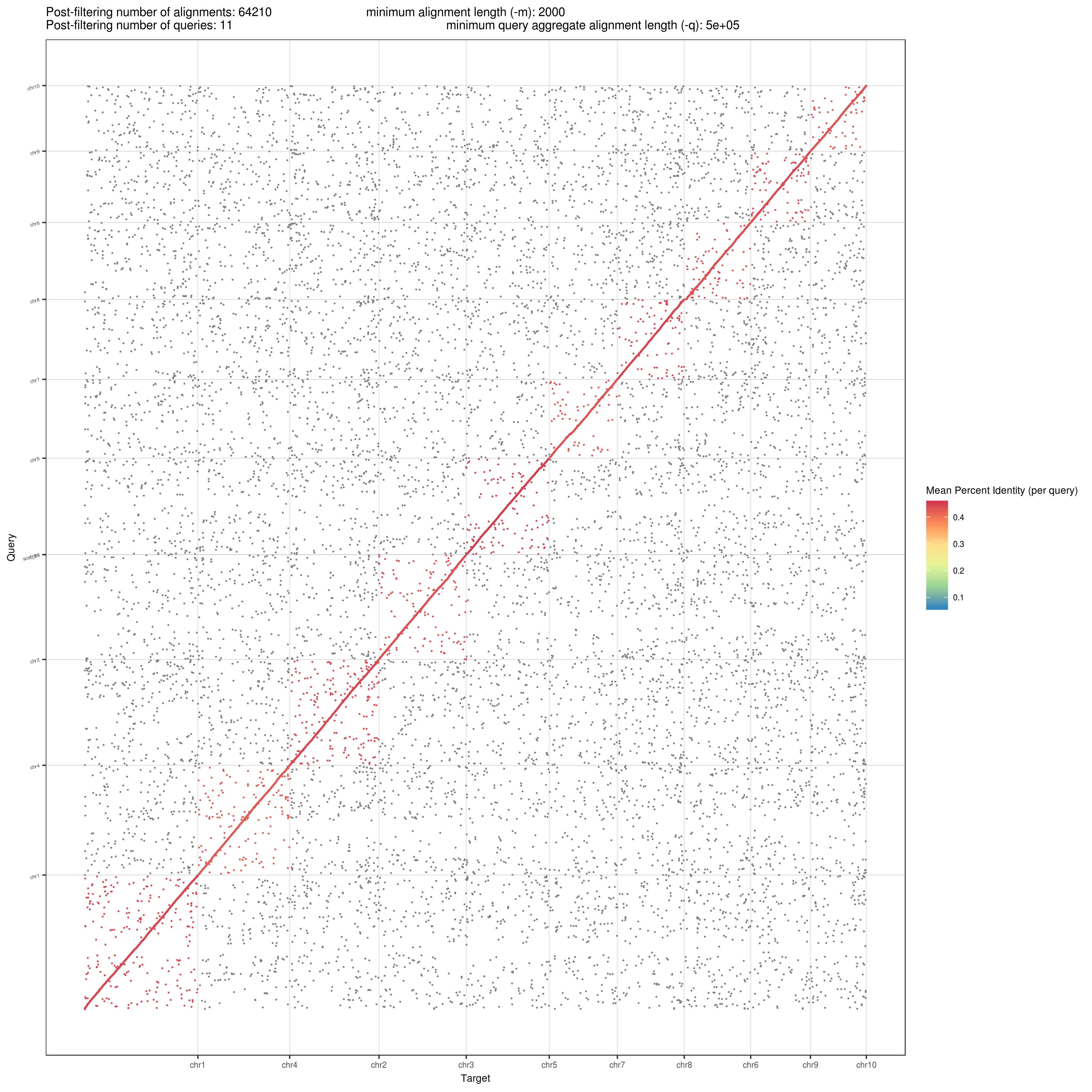
Figure 2: Dot Plot comparing the 2 genomes. Here, target is B73 V4 and query is CML247. You can rename the axis labels in the plot by modifying the code.