Visualize gaps in the genome
Visualize Gaps in Assemblies
The scaffold-level assemblies usually contain gaps and it is very important know how big and widespread these gaps are in order to evaluate the quality of an assembly. Here, in this tutorial, we will examine few publicly available maize genomes and plot the gaps in them.
Dataset
MaizeGDB has many different genomes available for download. For this tutorial, we will use the following 6 genomes.
- W22 cultivar of Zea mays subspp mays
- PI566673 cultivar of Zea mays subspp mexicana
- PH207 cultivar of Zea mays subspp mays
- Mo17 cultivar of Zea mays subspp mays
- CML247 cultivar of Zea mays subspp mays
- B73 cultivar of Zea mays subspp mays
Download
Download the files using the wget command and extract them using gunzip
1
2
3
4
5
6
7
8
wget https://ftp.maizegdb.org/MaizeGDB/FTP/Zm-B73-REFERENCE-GRAMENE-4.0/Zm-B73-REFERENCE-GRAMENE-4.0.fa.gz
wget https://ftp.maizegdb.org/MaizeGDB/FTP/Zm-CML247-REFERENCE-PANZEA-1.1/Zm-CML247-REFERENCE-PANZEA-1.1.fa.gz
wget https://ftp.maizegdb.org/MaizeGDB/FTP/Zm-Mo17-REFERENCE-CAU-1.0/Zm-Mo17-REFERENCE-CAU-1.0.fa.gz
wget https://ftp.maizegdb.org/MaizeGDB/FTP/Zm-PH207-REFERENCE_NS-UIUC_UMN-1.0/Zm-PH207-REFERENCE_NS-UIUC_UMN-1.0.fasta.gz
wget https://ftp.maizegdb.org/MaizeGDB/FTP/Zm-W22-REFERENCE-NRGENE-2.0/Zm-W22-REFERENCE-NRGENE-2.0.fasta.gz
wget https://ftp.maizegdb.org/MaizeGDB/FTP/Zx-PI566673-REFERENCE-YAN-1.0/Zx-PI566673-REFERENCE-YAN-1.0.fa.gz
module load parallel
parallel "gunzip {}" ::: *.gz
Gap Size calculations
Gaps are usually coded as N in the scaffolds. Normally, a fixed (constant) size denotes that there was a fusion of contigs/scaffolds based on some kind of evidence (genetic map or optical map). Though there is no standards set for various types of maps, BioNano uses 13 N gap, and most genetic map programs use 100 N gap.
To calculate the gaps, we will set up a script as follows:
get-N-sizes.sh
1
2
3
4
5
6
7
8
9
10
#!/bin/bash
genome="$1"
out=$(basename ${genome%.*})
module load bioawk
tr "ATGCatgc" "xxxxxxxx" < $genome |\
bioawk -c fastx '{print $seq}' | \
sed -e 's/xN/\nN/g' -e 's/Nx/N\n/g' | \
sed 's/x//g' | \
awk '{print length($1)}' |\
grep -vw "^0$" > ${out}_Nsizes.txt
Run it as:
1
2
3
for fasta in *.fasta; do
  ./get-N-sizes.sh $fasta;
done
You will get text files as output, we will process them to create data files to plot them in R.
1
2
3
4
5
6
7
8
9
10
11
12
13
14
15
16
# files with gaps for each line
for gaps in *.txt; do
  name=$(echo $gaps |cut -f 2 -d "-");
  awk -v x=$name  '{print x"\t"$0}' $gaps > ${names}-size.txt;
done
# combined file for gaps
cat *-size.txt > lines_info.txt
# add headers
for size in *-size.txt; do
  sed -i '1 i Line\tNsize' $size;
done
# total gap size per genome file
datamash groupby 1 sum 2 <lines_info.txt > total_gaps_bases.txt
# add headers
sed -i '1 i Line\tGapSize' lines_info.txt;
sed -i '1 i Lines\tTotalGapSize' lines_info.txt;
Now that we have all the files, we will plot them in R.
Plots
Gaps per maize line
Distribution of gaps per line to visualize how big and how frequent gaps are in the assemblies. Now the files are created, in the R terminal, run these commands.
1
2
3
4
5
6
7
8
9
10
size=read.table("B73-size.txt", header=TRUE)
png("b73.png", 1500, 1000, pointsize=20)
hist(size$Nsize, main="Gap Size (Ns) in B73",
     xlab="N size (bp)", ylab="Frequency",
     border="olivedrab",
     col="olivedrab3",
     xlim=c(100,1000000),
     las=1,
     breaks=500)
dev.off()
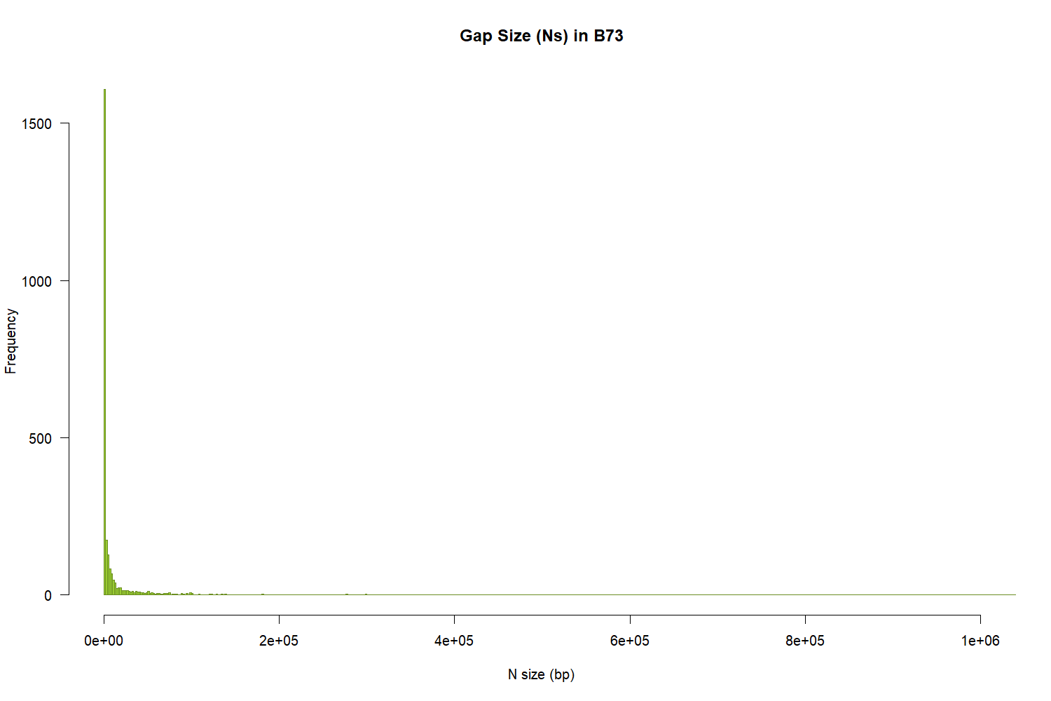
Figure 1: Gap size in B73
Total gaps in each maize line
Again, open the R terminal or R-Studio and enter these commands.
1
2
3
4
5
6
7
8
9
10
11
12
13
14
15
16
library(ggplot2)
theme_set(theme_bw())
gaps <- read.csv("lines_info.txt", sep="\t", stringsAsFactors=TRUE, header=TRUE)
ggplot(gaps, aes(Line, GapSize)) +
  geom_violin() +
  geom_jitter(aes(colour = Lines), shape=16, position=position_jitter(0.2)) +
  scale_y_continuous(trans='log10') +
  theme(axis.text.x = element_text(angle=90, vjust=0.6), legend.position="none") +
  labs(title="Gap Sizes in Maize genomes", x="Maize lines", y="Gap Sizes (bp)")
tgaps <- read.csv("total_gaps_bases.txt", sep="\t", stringsAsFactors=TRUE, header=TRUE)
barplot(tgaps$TotalGapSize, main="Total Gap Size (Ns) in Maize lines",
        names.arg=tgaps$Lines,
        ylab="Gaps (bp)",
        border="slateblue", col="slateblue3",
        las=3,
        ylim = range (0:500000000))
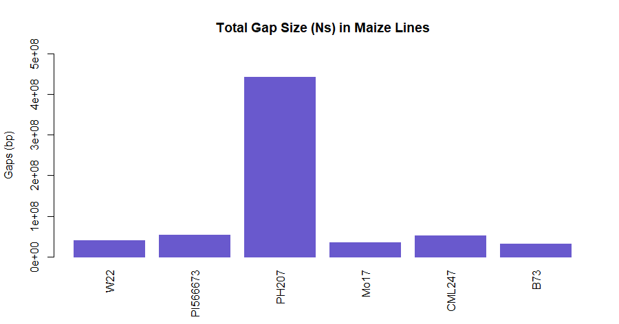
Figure 2: Total N (gap content) in Maize lines. Gaps for each maize line were summed together and is plotted as bar-graph.
Gap sizes in each maize line
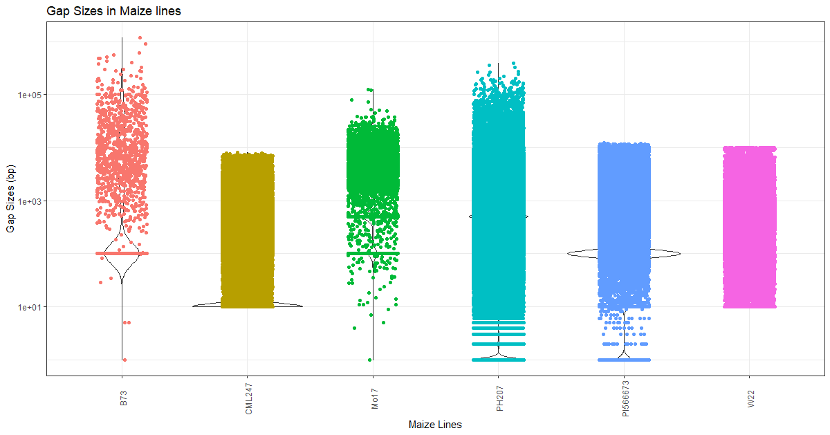
Figure 3: Gap size and distribution in each Maize line. Each dot represents a gap for that NAM line (x-axis) with the size identified in y-axis (bp). Note that the y axis labels are in log scale and is not linear (for making distributions even).