
FreeBayes variant calling workflow for DNA-Seq
Introduction
freebayes is a Bayesian genetic variant detector designed to find small polymorphisms, specifically SNPs (single-nucleotide polymorphisms), indels (insertions and deletions), MNPs (multi-nucleotide polymorphisms), and complex events (composite insertion and substitution events) smaller than the length of a short-read sequencing alignment (Garrison and Marth, 2012).
Dataset
For this tutorial we will use the dataset from BioProject PRJNA283785. This dataset has Illumina short reads for six different ecotypes of Arabidopsis thaliana (002185_Limeport-CC8070, 002186_Limeport-CC28464, 002187_Santa-Clara-CC8069, 002188_Santa-Clara-CC28722, 002189_Berkley-CC8068, 002190_Berkley-CC28067) and was originally used for re-evaluation of reported metal tolerance of Arabidopsis thaliana accessions. These reads were sequenced on Illumina HiSeq 2000, with genomic DNA (WGS), random selection, paired layout, library strategy,
Table 1: Dataset used for freebayes SNP calling.
| Run | SampleName | ReadPairs | TotalBases | ReadLength |
|---|---|---|---|---|
| SRR2032874 | 002185_Limeport-CC8070 | 17,116,111 | 4,922,884,384 | 287 |
| SRR2032873 | 002186_Limeport-CC28464 | 23,125,667 | 6,639,673,875 | 287 |
| SRR2032879 | 002187_Santa-Clara-CC8069 | 16,919,754 | 4,859,908,587 | 287 |
| SRR2032877 | 002188_Santa-Clara-CC28722 | 20,847,502 | 5,994,626,199 | 287 |
| SRR2032876 | 002189_Berkley-CC8068 | 18,613,942 | 5,348,144,580 | 287 |
| SRR2032875 | 002190_Berkley-CC28067 | 17,702,502 | 5,089,062,686 | 287 |
We will download the files as follows:
srr.ids
1
2
3
4
5
6
7
SRR2032874
SRR2032873
SRR2032879
SRR2032877
SRR2032876
SRR2032875
1
2
3
4
module load sra-toolkit
module load parallel
parallel -a srr.ids prefetch --max-size 50GB
parallel -a srr.ids fastq-dump --split-files --origfmt --gzip
Since reference genome of Arabidopsis is available here, we will use it as reference for mapping. We will have to download the genome from the database
1
2
3
4
5
wget ftp://ftp.ensemblgenomes.org/pub/plants/release-44/fasta/arabidopsis_thaliana/dna/Arabidopsis_thaliana.TAIR10.dna.toplevel.fa.gz
gunzip Arabidopsis_thaliana.TAIR10.dna.toplevel.fa.gz
# for qc you will need GFF file:
wget ftp://ftp.ensemblgenomes.org/pub/plants/release-44/gff3/arabidopsis_thaliana/Arabidopsis_thaliana.TAIR10.44.gff3.gz
gunzip Arabidopsis_thaliana.TAIR10.44.gff3.gz
These datasets are all we need to get started. Although, the SRA download through prefetch is faster, it takes long time for converting sra file to fastq using fastq-dump. Alternatively, you can obtain and download fastq files directly form European Nucleotide Archive (ENA). The links are saved here if you want to use them instead (note the IDs are different, but they are from the same study and the results will be identical regardless of what data you use)
Organization
The files and folders will be organized as follows:
1
2
3
4
5
6
7
8
9
10
11
12
13
14
15
16
17
18
19
20
21
22
freebayes
├── 0_index
│   └── Arabidopsis_thaliana.TAIR10.dna.toplevel.fa
├── 1_data
│   ├── SRR2032873_1.fastq.gz
│   ├── SRR2032873_2.fastq.gz
│   ├── SRR2032874_1.fastq.gz
│   ├── SRR2032874_2.fastq.gz
│   ├── SRR2032875_1.fastq.gz
│   ├── SRR2032875_2.fastq.gz
│   ├── SRR2032876_1.fastq.gz
│   ├── SRR2032876_2.fastq.gz
│   ├── SRR2032877_1.fastq.gz
│   ├── SRR2032877_2.fastq.gz
│   ├── SRR2032879_1.fastq.gz
│   ├── SRR2032879_2.fastq.gz
│   └── srr.ids
├── 2_fastqc
├── 3_mapping
├── 4_processing
├── 5_freebayes
└── 6_filtering
Overview
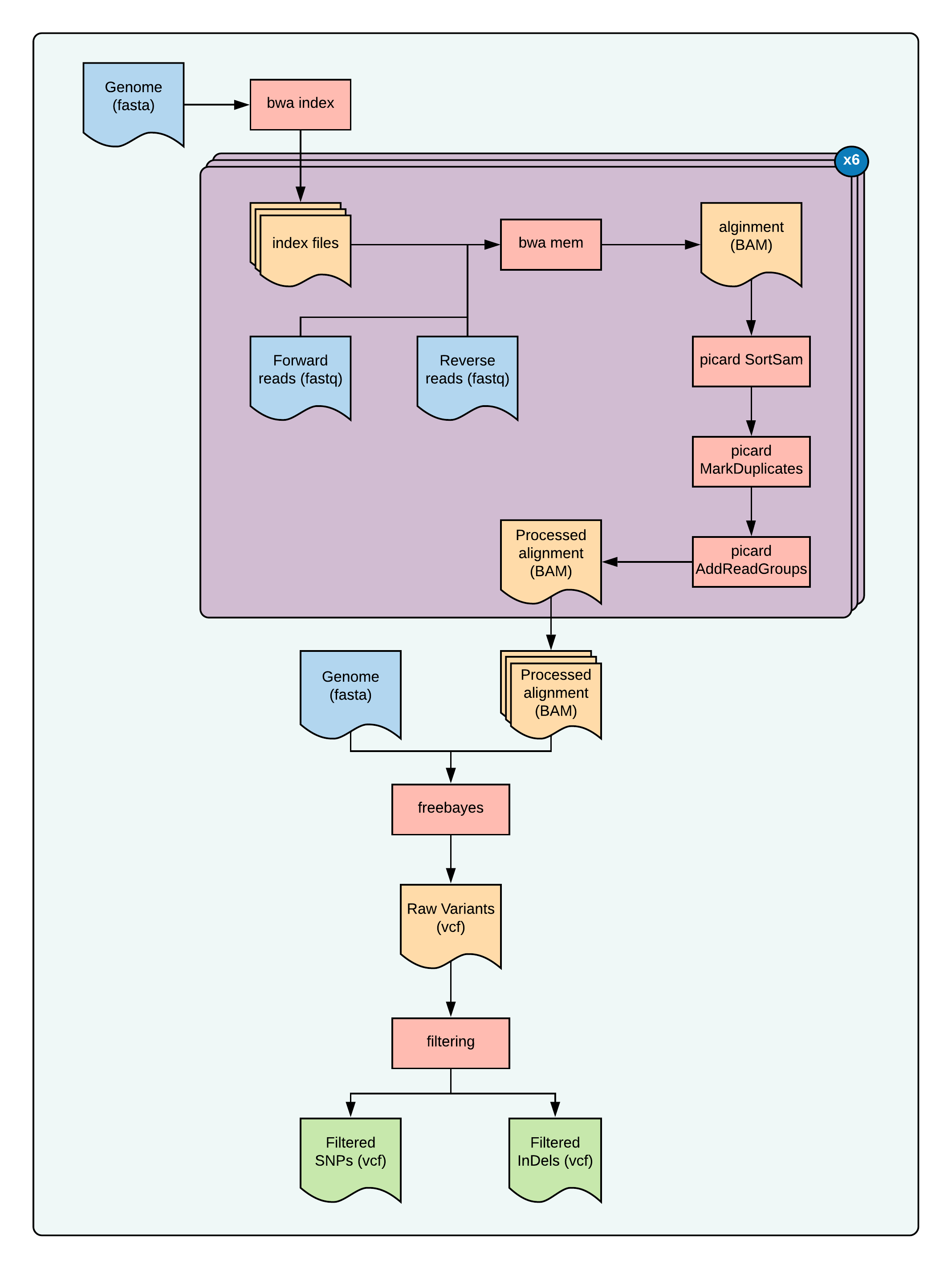 Fig 1: overview of this tutorial
Step 0: Quality check the files
Soft link the fastq files and run FASTQC on them:
1
2
3
4
5
6
7
cd 2_fastqc
for fq in ../1_data/*.fastq.gz; do
  ln -s $fastq
done
module load parallel
module load fastqc
parallel "fastqc {}"" ::: *.fastq
you can examine the results by opening each html page or you can merge them to a single report using multiqc. The data seems satisfactory, so we will proceed to next step.
Step 1: Map the raw reads to the genome
1
2
3
4
cd 3_mapping
for fq in ../1_data/*.fastq.gz; do
  ln -s $fq
done
Make a run script for alignment:
1
2
3
4
5
6
7
8
#!/bin/bash
genome=$1
read1=$2
read2=$3
out=$(echo $2 |sed 's/_1.fastq.gz/.bam/g')
module load bwa
module load samtools
bwa mem -M -t 16 $genome $read1 $read2 | samtools view -buS - > ${out}
Create commands:
1
2
3
4
5
for r1 in *_1.fastq.gz; do
  r2=$(echo $r1 |sed 's/_1.fastq.gz/_2.fastq.gz/g')
  genome="../0_index/Arabidopsis_thaliana.TAIR10.dna.toplevel.fa"
  echo "./runBWA.sh $genome $r1 $r2" ;
done > bwa.cmds
make SLURM scripts and submit
1
2
3
4
makeSLURMs.py 1 bwa.cmds
for sub in *.sub; do
  sbatch $sub;
done
Step 2: Process BAM files
In this step, we will sort the BAM files from previous step, add readgroups and mark duplicates in them.
Soft-link the files
1
2
3
4
cd 4_processing
for bam in ../3_mapping/*.bam; do
  ln -s $bam;
done
Make a run script for processing bam files
1
2
3
4
5
6
7
8
9
10
11
12
13
14
15
16
17
18
19
20
21
22
23
24
25
26
#!/bin/bash
bam=$1
name=$2
module load picard
module load samtools

picard SortSam \
      I=${bam} \
      O=${bam%.*}-sorted.bam \
      SORT_ORDER=coordinate

picard MarkDuplicates \
      I=${bam%.*}-sorted.bam \
      O=${bam%.*}-sorted-md.bam \
      M=${bam%.*}-md-metrics.txt

picard AddOrReplaceReadGroups \
      I=${bam%.*}-sorted-md.bam \
      O=${bam%.*}-sorted-md-rg.bam \
      RGID=${bam%.*} \
      RGLB=${name} \
      RGPL=illumina \
      RGPU=unit1 \
      RGSM=${name}

samtools index ${bam%.*}-sorted-md-rg.bam
you need a names.txt file with:
1
2
3
4
5
6
SRR2032874	Limeport-CC8070
SRR2032873	Limeport-CC28464
SRR2032879	Santa-Clara-CC8069
SRR2032877	Santa-Clara-CC28722
SRR2032876	Berkley-CC8068
SRR2032875	Berkley-CC28067
Now create commands:
1
2
3
while read a b; do
  echo "./runProcessing.sh ${a}.bam ${b}"
done > process.cmds
make SLURM scripts and submit
1
2
3
4
makeSLURMs.py 1 process.cmds
for sub in *.sub; do
  sbatch $sub;
done
Now we are ready to call SNPs on these bam files!
Step 3a: Run freebayes (single processor mode)
Next is to run the actual variant calling program, whcih is the freebayes. We run this on all your processed bam files (alignment data) simultaneously. This will generate a single VCF file. The default settings should work for most use cases, but if your samples are not diploid, then you need to set the --ploidy and adjust the --min-alternate-fraction accordingly.
1
2
3
4
cd 5_freebayes
for bam in ../4_processing/*-md-rg.bam*; do
  ln -s $bam;
done
Make a run script for freebayes (runFreeBayes.sh):
1
2
3
4
5
6
7
8
#!/bin/bash
ref="../0_index/Arabidopsis_thaliana.TAIR10.dna.toplevel.fa"
module load freebayes
ls *-md-rg.bam > bam.fofn
freebayes \
  --fasta-reference ${ref} \
  --bam-list bam.fofn \
  --vcf output.vcf \
make SLURM scripts and submit
1
2
3
echo "./runFreeBayes.sh" > freebayes.cmds
makeSLURMs.py 1 freebayes.cmds
sbatch freebayes_0.sub
When this completes, you will have the output.vcf file. This is your unfiltered raw variants file.
For the files above, it took > 5hrs to complete. Because of the design, the program runs only on a single processor.
1
2
3
real    320m1.051s
user    314m49.526s
sys     0m50.473s
Another alternative is to run them in small chunks, a stretch of genome, at a time. Although the program does not have threads option, it can be trivially parallelizable.
Step 3b: Run freebayes (processing small chunks of genome, in parallel)
Just like before, her run the freebayes but process the small chunks of genome at a time. Since freebayes can’t utilize multiple processors, you can run this processing step, many at a time, finishing the analyses faster. Fortunately, the included script does all this for you!
1
2
3
4
cd 6_freebayes-parallel
for bam in ../4_processing/*-md-rg.bam*; do
  ln -s $bam;
done
Make a run script for freebayes (runFreeBayesP.sh):
1
2
3
4
5
6
7
8
#!/bin/bash
ref="../0_index/Arabidopsis_thaliana.TAIR10.dna.toplevel.fa"
module load freebayes
ls *-md-rg.bam > bam.fofn
freebayes-parallel \
   <(fasta_generate_regions.py ${ref}.fai 100000) 16 \
   --fasta-reference ${ref} \
   --bam-list bam.fofn  > output.vcf
make SLURM scripts and submit
1
2
3
echo "./runFreeBayesP.sh" > freebayes.cmds
makeSLURMs.py 1 freebayes.cmds
sbatch freebayes_0.sub
Time take for this step:
1
2
3
real    66m29.306s
user    467m33.650s
sys     12m4.956s
As you can see, this takes a fraction of time as compared to the non-parallel approach. If you have a large genome and access to large clusters, this is clearly should be the way to go!
Step 4: filter the VCF file
In this final step, we will separate SNPs from InDels and do some plots to see how these variants are distributed. We will also do some filtering.
1
2
3
4
5
cd 7_filtering
ln -s ../6_freebayes-parallel/output.vcf
vcf=output.vcf
# generate stats
rtg vcfstats output.vcf > rtg_results-full.out
Table 1: RTG stats for the output VCF file:
| Sample_Name | Santa-Clara-CC8069 | Berkley-CC8068 | Santa-Clara-CC28722 | Limeport-CC28464 | Berkley-CC28067 | Limeport-CC8070 |
|---|---|---|---|---|---|---|
| SNPs | 15,481 | 14,597 | 14,173 | 14,269 | 14,623 | 14899 |
| MNPs | 2,320 | 2,349 | 2,262 | 2,318 | 2,303 | 2347 |
| Insertions | 2,207 | 2,123 | 2,086 | 2,152 | 2,190 | 2208 |
| Deletions | 3,686 | 3,636 | 3,579 | 3,470 | 3,825 | 3619 |
| Indels | 481 | 484 | 451 | 479 | 492 | 480 |
| Same_as_reference | 462,491 | 463,551 | 464,239 | 464,105 | 463,336 | 463167 |
| Missing_Genotype | 313 | 239 | 189 | 186 | 210 | 259 |
| SNP_Transitions/Transversions | 1.05 (8677/8242) | 1.07 (8278/7723) | 1.07 (8060/7556) | 1.07 (8086/7587) | 1.08 (8314/7721) | 1.06 (8373/7934 ) |
| Total_Het/Hom_ratio | 5.66 (20547/3628) | 5.41 (19571/3618) | 5.22 (18924/3627) | 5.31 (19091/3597) | 5.48 (19818/3615) | 5.56 (19961/3592) |
| SNP_Het/Hom_ratio | 9.96 (14068/1413) | 9.55 (13214/1383) | 8.97 (12751/1422) | 9.33 (12888/1381) | 9.51 (13232/1391) | 9.73 (13510/1389) |
| MNP_Het/Hom_ratio | 9.69 (2103/217) | 10.4 (2143/206) | 9.98 (2056/206) | 9.17 (2090/228) | 10.13 (2096/207) | 10.28 (2139/208) |
| Insertion_Het/Hom_ratio | 0.86 (1022/1185) | 0.76 (919/1204) | 0.77 (908/1178) | 0.81 (964/1188) | 0.84 (1003/1187) | 0.86 (1024/1184) |
| Deletion_Het/Hom_ratio | 4.34 (2996/690) | 4.16 (2932/704) | 4.09 (2876/703) | 4.15 (2796/674) | 4.42 (3119/706) | 4.24 (2929/690) |
| Indel_Het/Hom_ratio | 2.91 (358/123) | 3.00 (363/121) | 2.82 (333/118) | 2.8 (353/126) | 2.97 (368/124) | 2.97 (359/121) |
| Insertion/Deletion_ratio | 0.60 (2207/3686) | 0.58 (2123/3636) | 0.58 (2086/3579) | 0.62 (2152/3470) | 0.57 (2190/3825) | 0.61 (2208/3619) |
| Indel/SNP+MNP_ratio | 0.36 (6374/17801) | 0.37 (6243/16946) | 0.37 (6116/16435) | 0.37 (6101/16587) | 0.38 (6507/16926) | 0.37 (6307/17246) |
Next, we will perform some filtering. But first, more QC
1
2
3
4
# separate indels
vcftools --vcf $vcf --keep-only-indels --recode --recode-INFO-all --out output_indels-only.vcf
# separate SNPs
vcftools --vcf $vcf --remove-indels --recode --recode-INFO-all --out output_snps-only.vcf
QC plots:
1
2
ln -s ../0_index/Arabidopsis_thaliana.TAIR10.44.gff3
ln -s ../0_index/Arabidopsis_thaliana.TAIR10.dna.toplevel.fa
1
2
3
4
5
6
7
8
9
10
11
12
13
14
library(vcfR)
vcf <- read.vcfR( "output_snps-only.vcf.recode.vcf", verbose = FALSE )
dna <- ape::read.dna("Arabidopsis_thaliana.TAIR10.dna.toplevel.fa", format = "fasta")
gff <- read.table("Arabidopsis_thaliana.TAIR10.44.gff3", sep="\t", quote="")
chrom <- create.chromR(name='Supercontig', vcf=vcf, seq=dna, ann=gff)
png("quality.png", width = 10, height = 8, units = 'in', res = 300)
plot(chrom)
dev.off()
png("dotplots1.png", width = 10, height = 8, units = 'in', res = 300)
chromoqc(chrom, dp.alpha=20)
dev.off()
png("dotplot2.png", width = 10, height = 8, units = 'in', res = 300)
chromoqc(chrom, xlim=c(1.25e+07, 1.75e+07))
dev.off()
The plots:
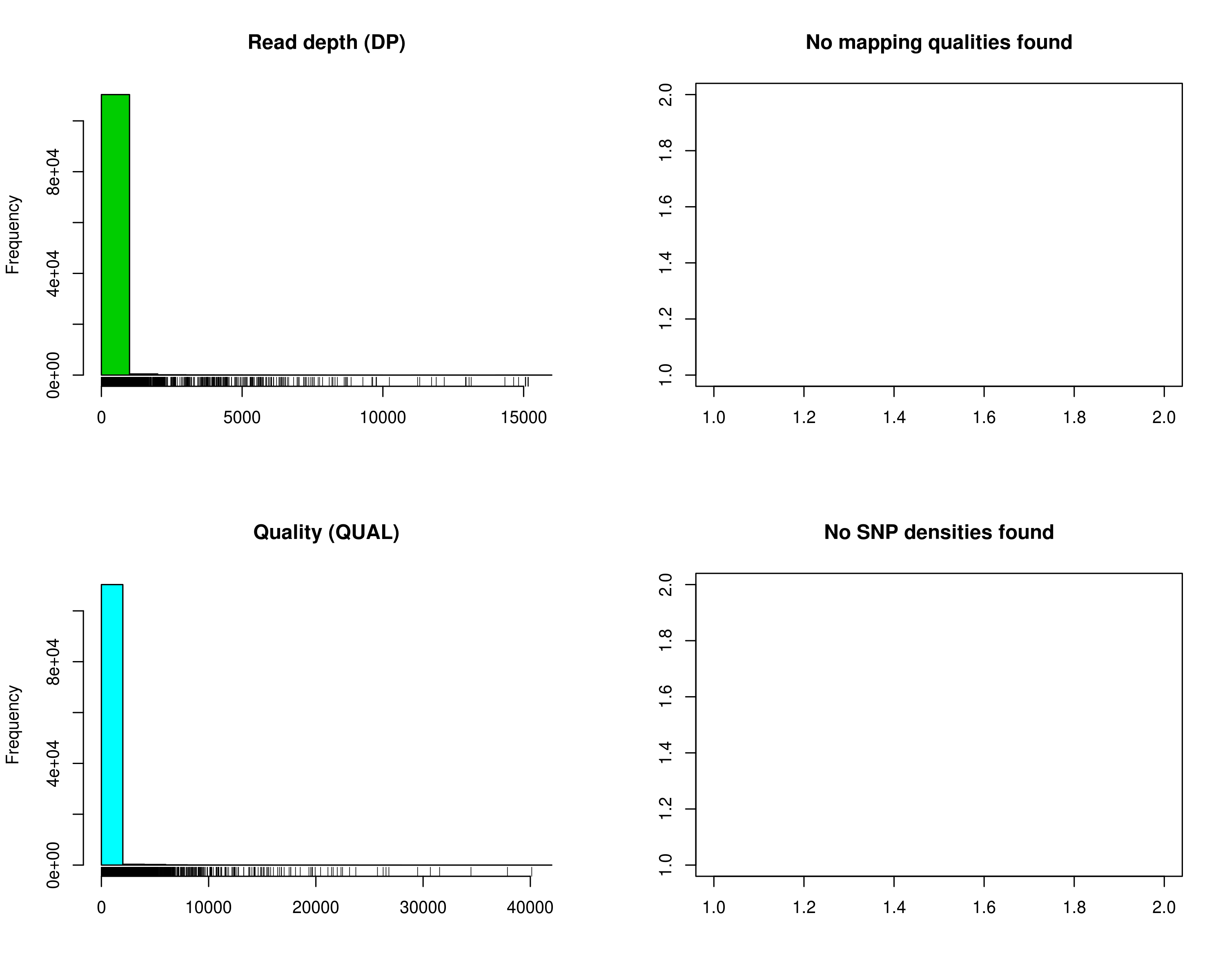 Fig 2: SNP quality distribution
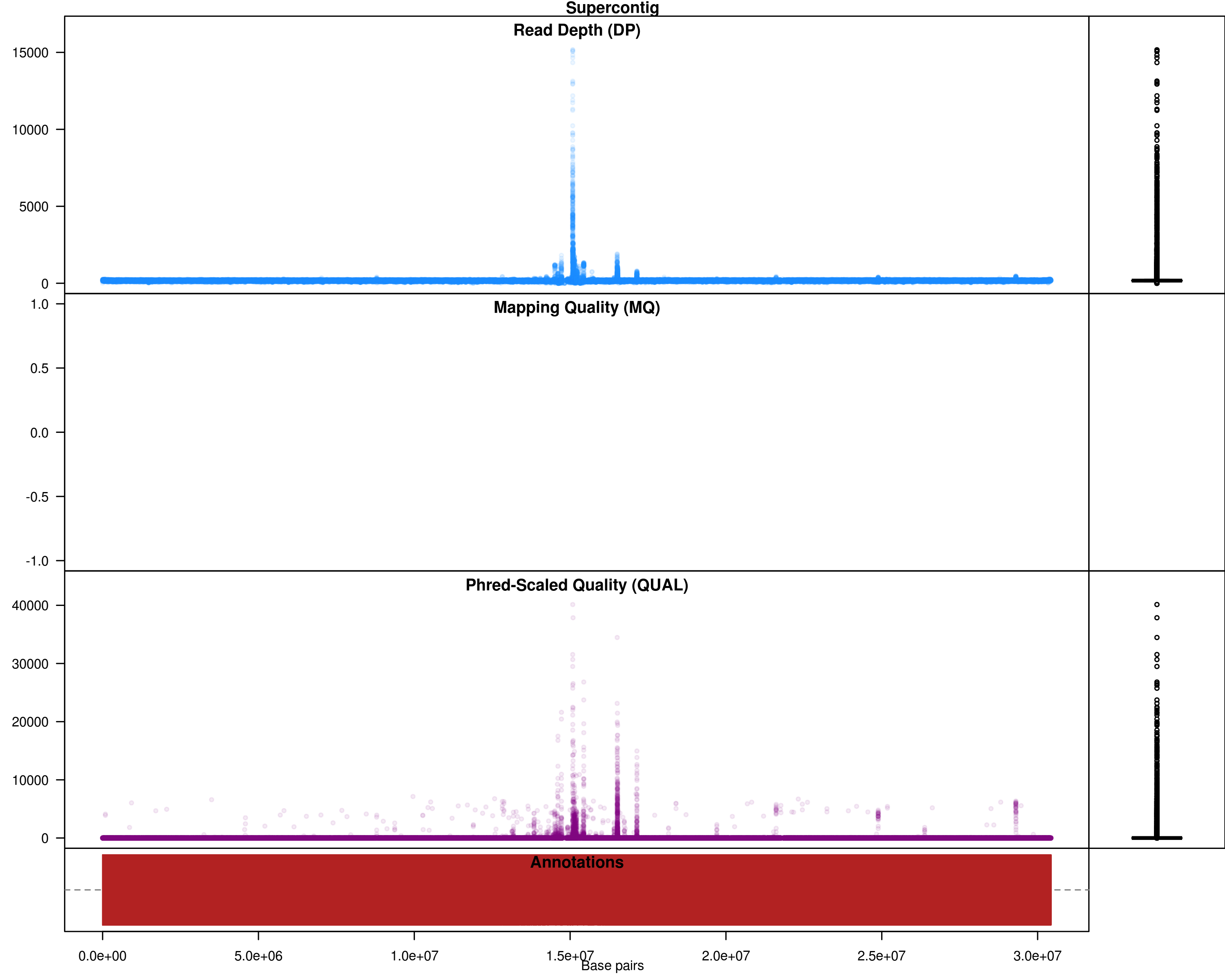 Fig 3: SNPs across the genome, with DP and quality values
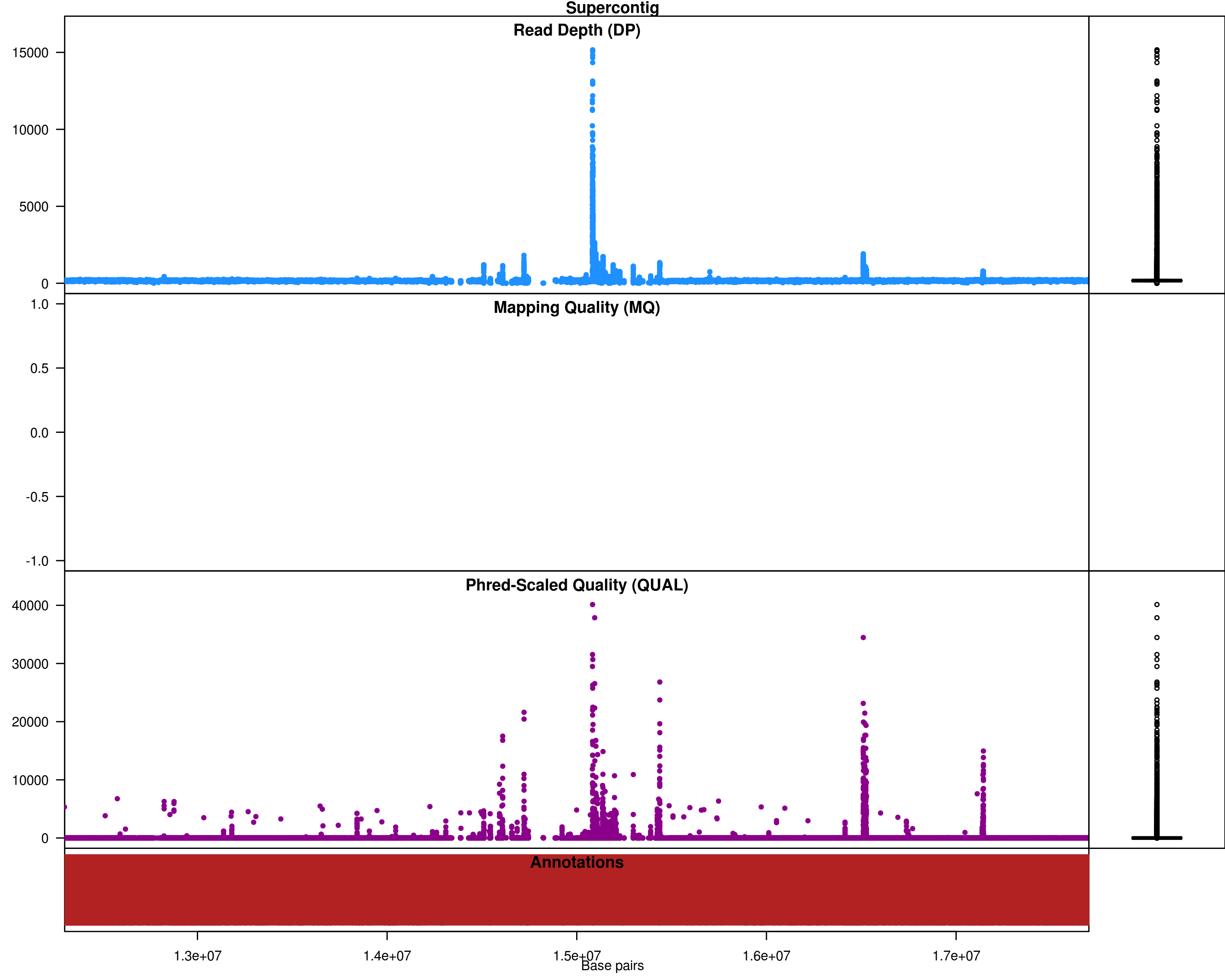 Fig 3: SNPs across the genome, with DP and quality values (zoomed in)
Based on the plots, the lines compared here are very similar to reference and they only differ in a small section of genome. The number of SNPs is very less as a result. No filtering is necessary, but if you wish to do some filtering:
1
2
3
4
5
6
7
8
9
module load vcftools
vcf=output_snps-only.vcf.recode.vcf
vcftools --vcf $vcf \
   --max-missing 1 \
   --mac 3 \
   --minQ 30 \
   --recode \
   --recode-INFO-all \
   --out output_snps-only_max_missing_1_mac_3_minq_30
stdout
1
2
3
4
5
6
7
8
9
10
11
12
13
14
15
16
VCFtools - 0.1.14
(C) Adam Auton and Anthony Marcketta 2009

Parameters as interpreted:
        --vcf output_snps-only.vcf.recode.vcf
        --recode-INFO-all
        --mac 3
        --minQ 30
        --max-missing 1
        --out output_snps-only_max_missing_1_mac_3_minq_30
        --recode

After filtering, kept 6 out of 6 Individuals
Outputting VCF file...
After filtering, kept 7871 out of a possible 449822 Sites
Run Time = 4.00 seconds
After filtering, you have 7871 SNPs that are present in all individuals and are non-monomorphic.