Introduction
Cell Ranger is a popular software package developed by 10x Genomics for the analysis of single-cell RNA sequencing (scRNA-seq) data. It provides a suite of tools for processing raw sequencing data, mapping reads to a reference genome, and quantifying gene expression at the level of individual cells. Here is a brief overview of the Cell Ranger pipeline:
- Demultiplexing: The first step in the pipeline involves demultiplexing the sequencing data, which separates reads from different samples or cell barcodes. This step also includes the identification of the unique molecular identifiers (UMIs) that are used to distinguish between different mRNA molecules from the same gene within a single cell.
- Read alignment: The demultiplexed reads are then aligned to a reference genome using the STAR aligner. This step allows the identification of the genomic location of each read and its associated UMI.
- Barcode processing: The next step involves the processing of the cell barcodes and UMIs. This includes the removal of potential sources of error such as low-quality barcodes, sequencing errors, and PCR duplicates.
- Gene expression quantification: The final step involves the quantification of gene expression at the level of individual cells. This is done by counting the number of UMIs associated with each gene in each cell, and normalizing the counts based on the total number of UMIs in each cell.
After the pipeline is complete, Cell Ranger provides several outputs, including gene expression matrices, quality control metrics, and visualization tools for exploring the data. Researchers can use these outputs to identify cell types, infer developmental trajectories, and analyze the heterogeneity of gene expression within and between cell populations.
Software Installation
- Cellranger from 10xgenomics. Install is unnecessary, as it is essentially a container
1
2
wget https://support.10xgenomics.com/single-cell-gene-expression/software/downloads/latest
tar -zxvf cellranger-7.1.0.tar.gz
- The only dependency for Cellranger is bcl2fastq. Mine was already installed on my HPC. Here is a link to the website
bcl2fastq - Suerat R package
Seurat
Be aware that there are boat-loads of dependencies for Suerat, which is fine if installing on a local PC. If on a cluster, I recommend asking an administrator to install it. - Install Genometools
I was lucky in that this module existed for my HPC. Here is a link to the website for download.
Genometools
An example using C. robusta/C. intestinalis SRA data
Get the data
1
2
3
4
5
6
7
8
9
10
11
12
13
14
15
16
17
18
19
20
21
22
23
24
25
26
#/work/GIF/remkv6/USDA/20_CellRanger/01_FromFastq
module load sra-toolkit/2.8.2-1-inqpbuz

##get the reads
fastq-dump --split-files --origfmt --gzip SRR8111691
fastq-dump --split-files --origfmt --gzip SRR8111692
fastq-dump --split-files --origfmt --gzip SRR8111693
fastq-dump --split-files --origfmt --gzip SRR8111694

##get the genome and unzip
#From a tunicate database 1,274 scafs.  I did not use as this I couldn't find gff. #hint, hint
wget http://hgdownload.soe.ucsc.edu/goldenPath/ci3/bigZips/ci3.fa.gz

##genome from ncbi with a matching gff
wget ftp://ftp.ncbi.nlm.nih.gov/genomes/all/GCF/000/224/145/GCF_000224145.3_KH/GCF_000224145.3_KH_genomic.fna.gz
gunzip GCF_000224145.3_KH_genomic.fna.gz

##get the gene gff for genome (NCBI) -- its assembly has 1280 scaffolds.
wget ftp://ftp.ncbi.nlm.nih.gov/genomes/all/GCF/000/224/145/GCF_000224145.3_KH/GCF_000224145.3_KH_genomic.gff.gz
gunzip  GCF_000224145.3_KH_genomic.gff.gz

##CellRanger will not accept the GFF format, so you'll need to convert it to to gtf.  This is easily done with genometools
#genometools doesnt like anything but the standard naming conventions in the column 3 of the gff, so all of those were skipped (pseudogenes, snoRNAs, etc).  If you want all of this, you can change the column 3 to gene, and they can be included in the gtf.  Another thing to consider is to change the mitochondrial gene names to contain a unique ID from genomic genes(  i.e.  Change gene1 to MT-gene1 )

module load genometools
gt gff3_to_gtf GCF_000224145.3_KH_genomic.gff >GCF_000224145.3_KH_genomic.gtf
Prepare gtf, genome, and reads
1
2
3
4
5
6
7
8
9
10
11
12
13
14
15
16
17
18
19
20
21
22
23
24
25
26
##Prepare both the gtf and the genome fasta.
#Be aware that whatever is in column 9 of the gtf after ID=, will be the name of your genes in the analysis.

module load bcl2fastq2/2.20.0.422-py2-bpx6pnb

cellranger-3.0.2/cellranger mkgtf GCF_000224145.3_KH_genomic.gtf GCF_000224145.3_KH_genomicfiltered.gtf
cellranger-3.0.2/cellranger mkref --genome C_robusta --fasta=GCF_000224145.3_KH_genomic.fna --genes=GCF_000224145.3_KH_genomic.gtf --ref-version=3.0.0


##Now when specifiying the reference I can use this.
###cellranger --transcriptome=/work/GIF/remkv6/USDA/20_CellRanger/01_CionaRobusta/C_robusta

#Witholding download times, this takes a few minutes.


#need to rename your fastq files so tha they fit this format.
#_L00#_  represents lane number
mv  SRR8111691_1.fastq.gz SRR8111691_S1_L001_R1_001.fastq.gz
mv  SRR8111691_2.fastq.gz SRR8111691_S1_L001_R2_001.fastq.gz
mv  SRR8111692_1.fastq.gz SRR8111692_S1_L002_R1_001.fastq.gz
mv  SRR8111692_2.fastq.gz SRR8111692_S1_L002_R2_001.fastq.gz
mv  SRR8111693_1.fastq.gz SRR8111693_S1_L003_R1_001.fastq.gz
mv  SRR8111693_2.fastq.gz SRR8111693_S1_L003_R2_001.fastq.gz
mv  SRR8111694_1.fastq.gz SRR8111694_S1_L004_R1_001.fastq.gz
mv  SRR8111694_2.fastq.gz SRR8111694_S1_L004_R2_001.fastq.gz
Run Cellranger Count
1
2
3
4
5
#Since these were part of the same GEM well, I can treat them all as one sample (i.e. put all SRA files in comma delimited list). --id is just a made up name for the experiment
cellranger-3.0.2/cellranger count --id=testsra  --sample=SRR8111691,SRR8111692,SRR8111693,SRR8111694 --fastqs=/work/GIF/remkv6/USDA/20_CellRanger/01_CionaRobusta/fastq/  --transcriptome=/work/GIF/remkv6/USDA/20_CellRanger/01_CionaRobusta/C_robusta

# This took 2 hours with 16cpus 124Gb ram, a 115Mb genome and 26.7 Gigabases of data
Cellranger count output
1
2
#/work/GIF/remkv6/USDA/20_CellRanger/01_CionaRobusta/testsra/outs
If you go down a couple directores to outs, this is where your data output is.  The files in outs can be further analyzed using Suerat.  However, the first thing to look at is the preliminary output in web_summary.html. The last 20 or so lines of your stdout should tell you exactly the path to the outs/directory.
1
2
3
4
5
6
7
8
9
10
11
12
13
14
15
16
17
18
Here is the content of the "outs" folder. Results can get you straight to the differentially expressed genes among your cells, a pca plot, and a tsne plot.
34M Feb 27 18:22 raw_feature_bc_matrix.h5
  5 Feb 27 18:23 raw_feature_bc_matrix/
5.0M Feb 27 18:24 filtered_feature_bc_matrix.h5
  5 Feb 27 18:24 filtered_feature_bc_matrix/
6.9G Feb 27 18:26 possorted_genome_bam.bam
107M Feb 27 18:28 molecule_info.h5
1.6M Feb 27 18:29 possorted_genome_bam.bam.bai
  6 Feb 27 18:30 analysis/
3.6M Feb 27 18:32 web_summary.html
646 Feb 27 18:32 metrics_summary.csv
23M Feb 27 18:33 cloupe.cloupe


To use Seurat, you'll the raw data, found in  in testsra/outs/raw_feature_bc_matrix/
You'll need to gunzip each file and rename features.tsv to genes.tsv.
Begin secondary analysis with Suerat
1
2
3
4
5
6
7
8
9
10
11
12
13
14
15
16
17
18
19
20
21
22
23
24
25
26
27
28
29
30
31
32
33
34
35
36
37
38
39
40
41
42
43
44
45
46
module load r/3.5.0-py2-x335hrh
module load hdf5
module load r-dplyr/0.7.5-py2-r3.5-4jcgekn
#My directory
#/work/GIF/remkv6/USDA/20_CellRanger/01_CionaRobusta/testsra/outs/raw_feature_bc_matrix
for f in *; do gunzip $f;done
mv features.tsv genes.tsv
#load required libraries
library(Seurat)
library(dplyr)
#Load in the required files (barcodes.tsv, genes.tsv, and matrix.mtx), from the raw data files (raw_feature_bc_matrix).
CionaBrain.data <- Read10X(data.dir = "/work/GIF/remkv6/USDA/20_CellRanger/01_CionaRobusta/testsra/outs/raw_feature_bc_matrix")
# This has something to do with matrix sizes and memory usage.
dense.size <- object.size(x = as.matrix(x = CionaBrain.data))
dense.size
################################################################################
80966018792 bytes
################################################################################
sparse.size <- object.size(x = CionaBrain.data)
sparse.size
################################################################################
295497328 bytes
################################################################################
dense.size/sparse.size
################################################################################
274 bytes
################################################################################
## Use the raw data to remove genes expressed in fewer than 4 cells and remove all cells with fewer than 200 genes.
CionaBrain <- CreateSeuratObject(raw.data = CionaBrain.data, min.cells = 3, min.genes = 200, project = "CionaBrain")
#Normally you'd grab the mitochondrial genes and remove them. It looks like the seurat tutorial greps for an MT in the gene name for human pbc.)
#this did not work, and there were not any mitochondrial genes in the genes.tsv anyway. #suspicious
#mito.genes <- grep(pattern = "MT-", x = rownames(x = CionaBrain@data), value = TRUE)
#percent.mito <- Matrix::colSums(CionaBrain@raw.data[mito.genes, ])/#Matrix::colSums(CionaBrain@raw.data)
#CionaBrain <- AddMetaData(object = CionaBrain, metadata = percent.mito, col.name = "percent.mito")
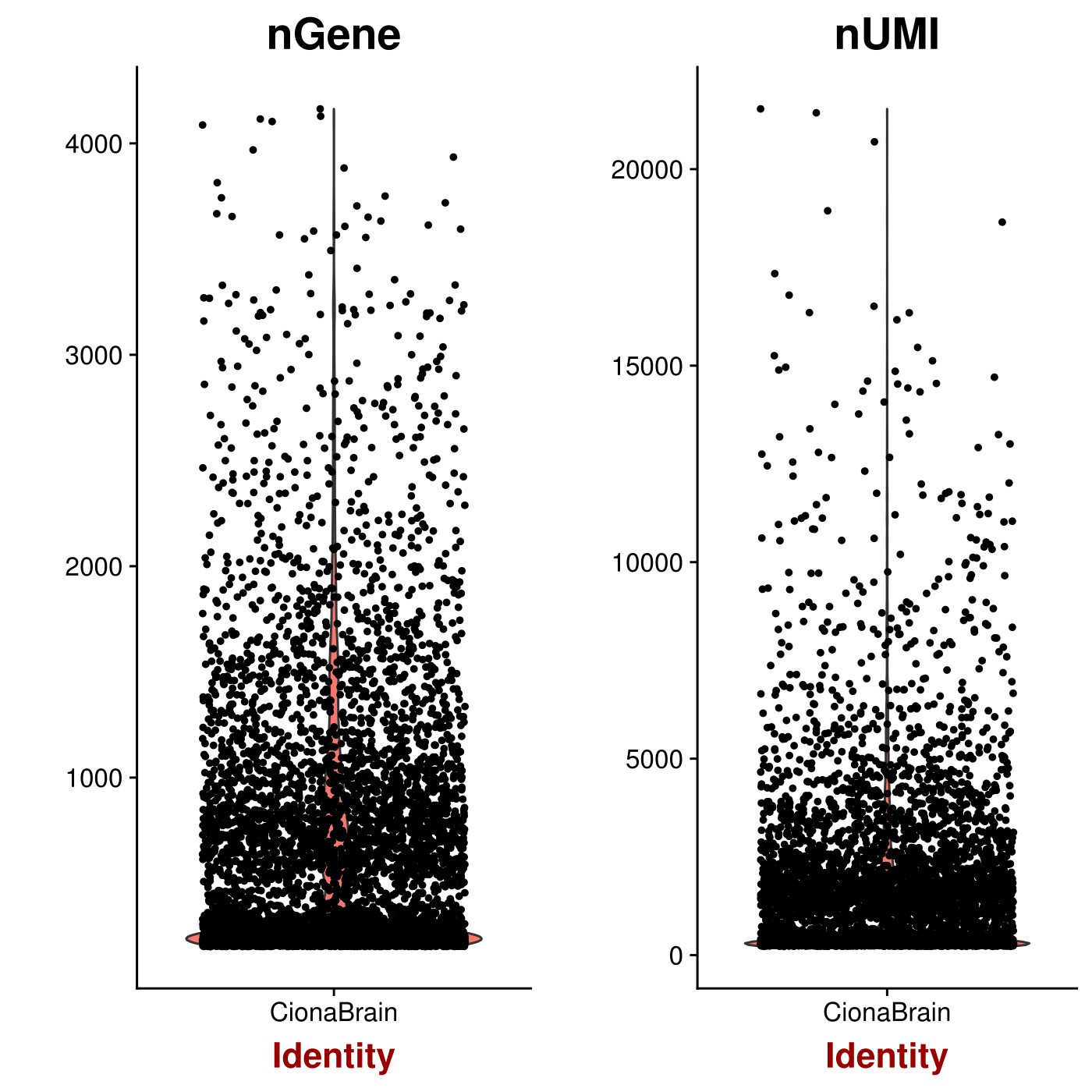
#Save a violin plot and view potential outliers for possible cell doublets
pdf(file = "/work/GIF/remkv6/USDA/20_CellRanger/01_CionaRobusta/testsra/outs/Violin.pdf")
VlnPlot(object = CionaBrain, features.plot = c("nGene", "nUMI"), nCol = 2)
dev.off()
1
2
3
4
5
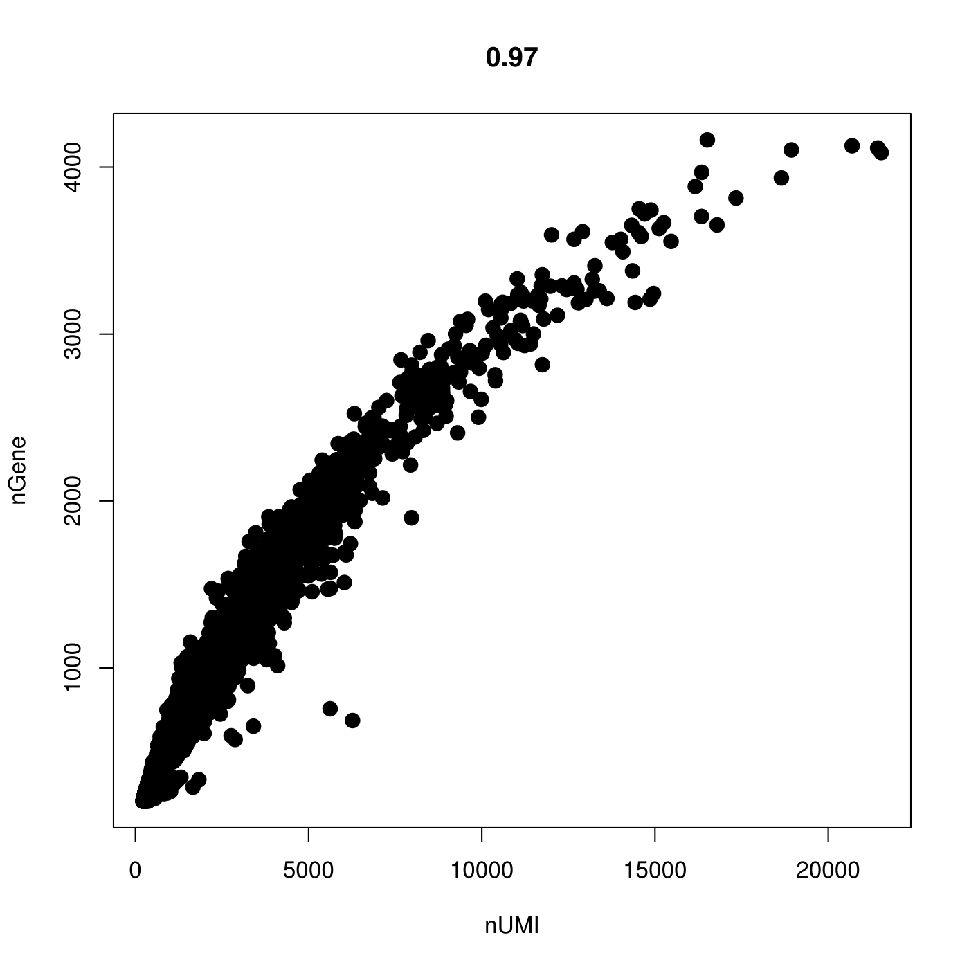
#plot number of genes vs number of UMI, another way to filter outliers for doublets etc.
pdf(file = "/work/GIF/remkv6/USDA/20_CellRanger/01_CionaRobusta/testsra/outs/GenesVsUMI.pdf")
par(mfrow = c(1, 1))
GenePlot(object = CionaBrain, gene1 = "nUMI", gene2 = "nGene")
dev.off()
1
2
3
4
5
6
7
8
9
10
#remove cells that have unique gene counts over 2200 (potential doublets) and less than 200(low depth/ambient RNA?)
CionaBrain <- FilterCells(object = CionaBrain, subset.names = c("nGene", "percent.mito"), low.thresholds = c(200, -Inf), high.thresholds = c(2200, 0.05))
#Normalize the data
CionaBrain <- NormalizeData(object = CionaBrain, normalization.method = "LogNormalize", scale.factor = 10000)
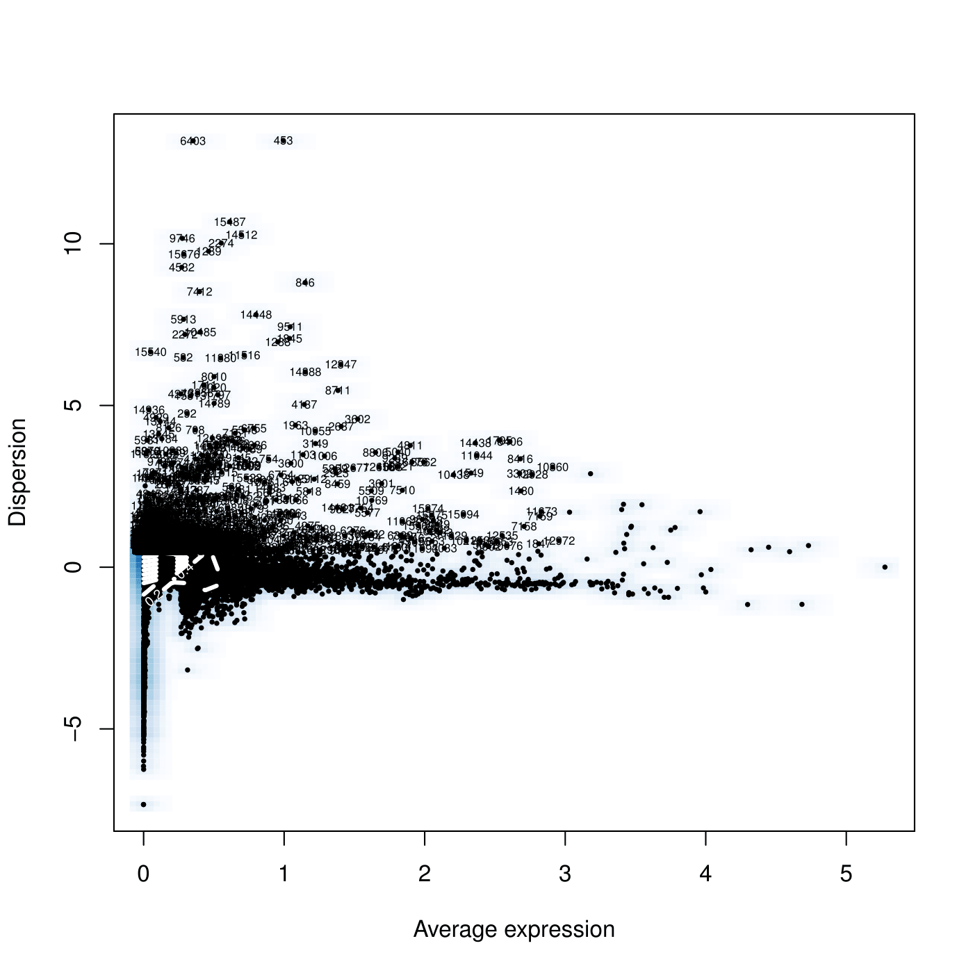
#Detect variable genes across the single cells
pdf(file = "/work/GIF/remkv6/USDA/20_CellRanger/01_CionaRobusta/testsra/outs/DispersionVsExpression.pdf")
CionaBrain <- FindVariableGenes(object = CionaBrain, mean.function = ExpMean, dispersion.function = LogVMR, x.low.cutoff = 0.0125, x.high.cutoff = 3, y.cutoff = 0.5)
dev.off()
1
2
3
4
5
6
7
8
9
10
11
12
13
14
15
16
17
18
19
20
21
22
23
24
25
26
27
28
29
30
31
32
33
34
35
36
37
38
39
40
41
42
43
44
45
46
47
48
49
50
51
52
53
54
55
56
57
58
59
60
61
62
63
64
65
66
67
68
69
70
71
72
73
74
75
76
77
78
79
80
length(x = CionaBrain@var.genes)
[1] 1910
#Scale the data
CionaBrain <- ScaleData(object = CionaBrain, vars.to.regress = c("nUMI"))
#note, my gene names are numbers. That is what is represented here.
CionaBrain <- RunPCA(object = CionaBrain, pc.genes = CionaBrain@var.genes, do.print = TRUE, pcs.print = 1:5, genes.print = 5)
################################################################################
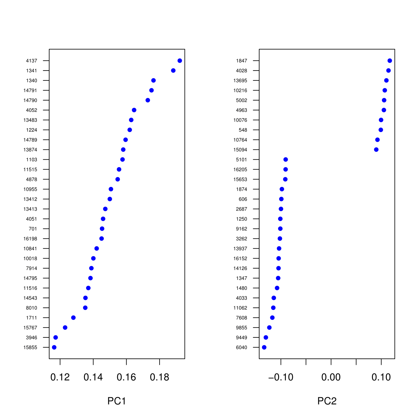
[1] "PC1"
[1] "1847" "4963" "4028" "13695" "5002"
[1] ""
[1] "4137" "1341" "1340" "14791" "14790"
[1] ""
[1] ""
[1] "PC2"
[1] "6040" "9449" "9855" "7608" "11062"
[1] ""
[1] "1847" "4028" "13695" "10216" "5002"
[1] ""
[1] ""
[1] "PC3"
[1] "4679" "14698" "7162" "2274" "15487"
[1] ""
[1] "1847" "4028" "4963" "548" "10764"
[1] ""
[1] ""
[1] "PC4"
[1] "1847" "4028" "13695" "4963" "548"
[1] ""
[1] "8046" "5862" "4411" "221" "13988"
[1] ""
[1] ""
[1] "PC5"
[1] "7608" "1347" "2687" "606" "9162"
[1] ""
[1] "12199" "14383" "8545" "7165" "10221"
[1] ""
[1] ""
################################################################################
PrintPCA(object = CionaBrain, pcs.print = 1:5, genes.print = 5, use.full = FALSE)
################################################################################
[1] "PC1"
[1] "1847" "4963" "4028" "13695" "5002"
[1] ""
[1] "4137" "1341" "1340" "14791" "14790"
[1] ""
[1] ""
[1] "PC2"
[1] "6040" "9449" "9855" "7608" "11062"
[1] ""
[1] "1847" "4028" "13695" "10216" "5002"
[1] ""
[1] ""
[1] "PC3"
[1] "4679" "14698" "7162" "2274" "15487"
[1] ""
[1] "1847" "4028" "4963" "548" "10764"
[1] ""
[1] ""
[1] "PC4"
[1] "1847" "4028" "13695" "4963" "548"
[1] ""
[1] "8046" "5862" "4411" "221" "13988"
[1] ""
[1] ""
[1] "PC5"
[1] "7608" "1347" "2687" "606" "9162"
[1] ""
[1] "12199" "14383" "8545" "7165" "10221"
[1] ""
[1] ""
################################################################################
#Visualize principal components
pdf(file = "/work/GIF/remkv6/USDA/20_CellRanger/01_CionaRobusta/testsra/outs/VizPCA.pdf")
VizPCA(object = CionaBrain, pcs.use = 1:2)
dev.off()
1
2
3
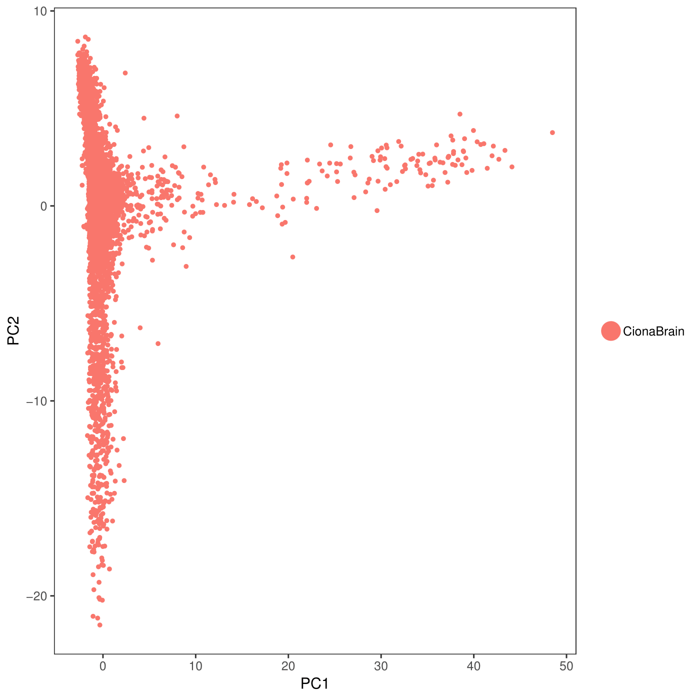
pdf(file = "/work/GIF/remkv6/USDA/20_CellRanger/01_CionaRobusta/testsra/outs/UnlabeledPCA.pdf")
PCAPlot(object = CionaBrain, dim.1 = 1, dim.2 = 2)
dev.off()
1
2
3
4
5
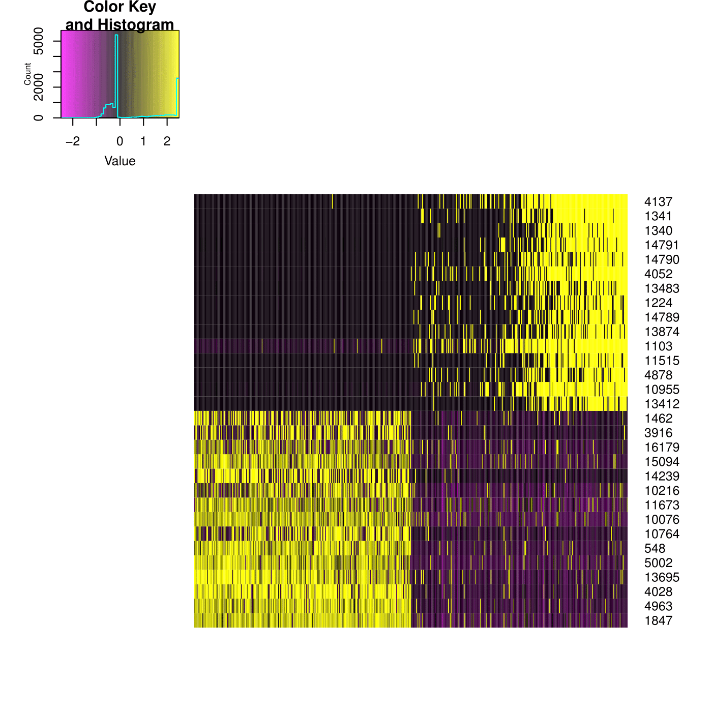
#create a heat map of principle components
CionaBrain <- ProjectPCA(object = CionaBrain, do.print = FALSE)
pdf(file = "/work/GIF/remkv6/USDA/20_CellRanger/01_CionaRobusta/testsra/outs/PCHeatmap.pdf")
PCHeatmap(object = CionaBrain, pc.use = 1, cells.use = 500, do.balanced = TRUE, label.columns = FALSE)
dev.off()
1
2
3
4
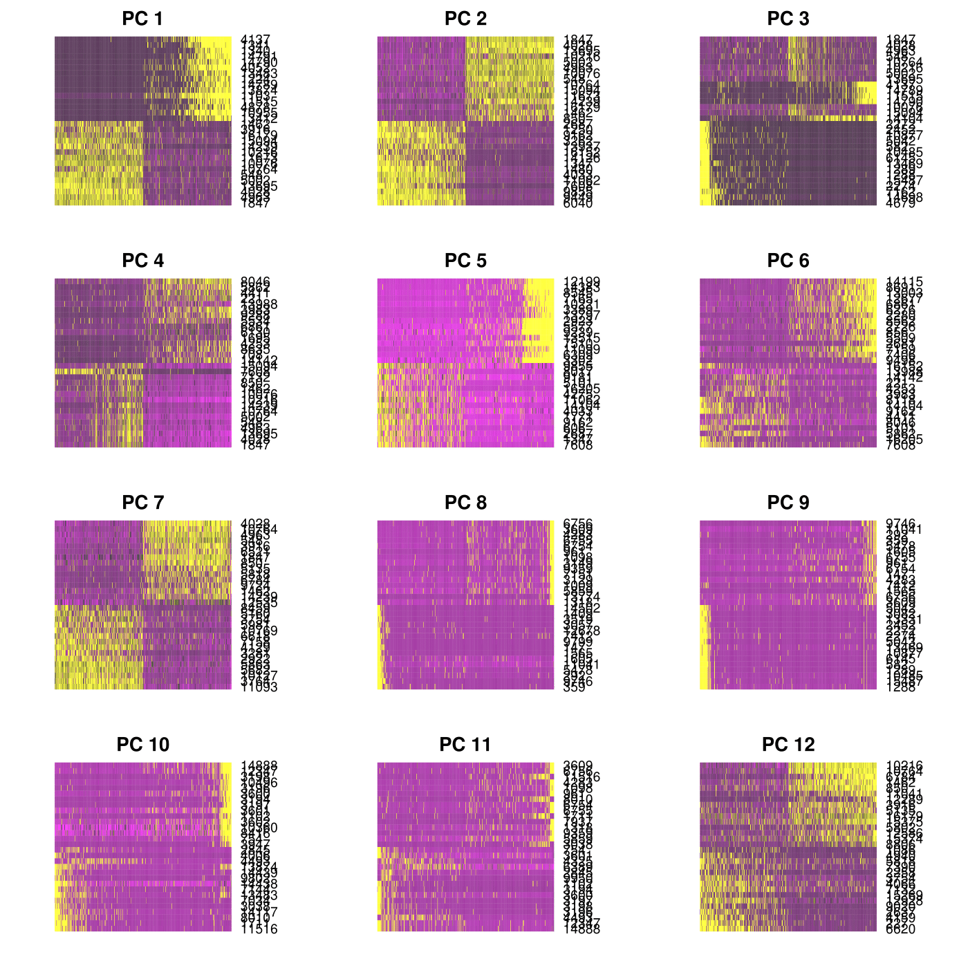
#Plot multiple PC heatmaps
pdf(file = "/work/GIF/remkv6/USDA/20_CellRanger/01_CionaRobusta/testsra/outs/MultPCHeatmap.pdf")
PCHeatmap(object = CionaBrain, pc.use = 1:12, cells.use = 500, do.balanced = TRUE, label.columns = FALSE, use.full = FALSE)
dev.off()
1
2
3
4
5
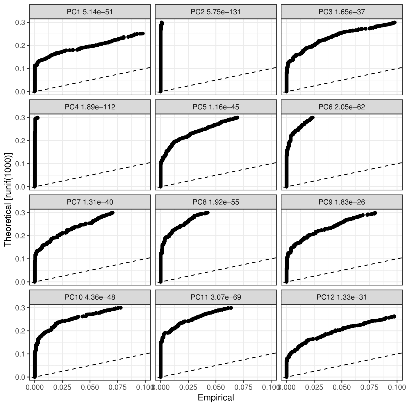
#Which of your PC are significant? all 12 of mine were significant.
CionaBrain <- JackStraw(object = CionaBrain, num.replicate = 100, display.progress = FALSE)
pdf(file = "/work/GIF/remkv6/USDA/20_CellRanger/01_CionaRobusta/testsra/outs/JackStrawPlot.pdf")
JackStrawPlot(object = CionaBrain, PCs = 1:12)
dev.off()
1
2
3
4
5
6
7
8
9
10
11
12
13
14
15
16
17
18
19
20
21
22
23
24
CionaBrain <- FindClusters(object = CionaBrain, reduction.type = "pca", dims.use = 1:12, resolution = 0.6, print.output = 0, save.SNN = TRUE)
PrintFindClustersParams(object = CionaBrain)
################################################################################
Parameters used in latest FindClusters calculation run on: 2019-02-28 14:42:16
=============================================================================
Resolution: 0.6
-----------------------------------------------------------------------------
Modularity Function Algorithm n.start n.iter
1 1 100 10
-----------------------------------------------------------------------------
Reduction used k.param prune.SNN
pca 30 0.0667
-----------------------------------------------------------------------------
Dims used in calculation
=============================================================================
1 2 3 4 5 6 7 8 9 10 11 12
################################################################################
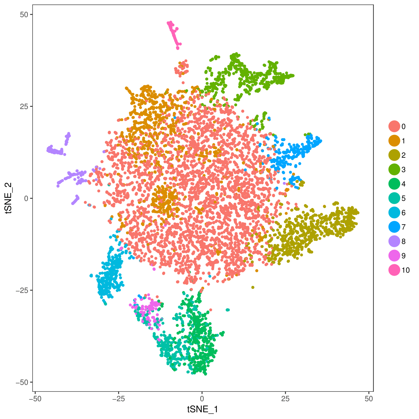
# Create TSNE plot
CionaBrain <- RunTSNE(object = CionaBrain, dims.use = 1:10, do.fast = TRUE)
pdf(file = "/work/GIF/remkv6/USDA/20_CellRanger/01_CionaRobusta/testsra/outs/TSNEPlot.pdf")
TSNEPlot(object = CionaBrain)
dev.off()
Sources
How to run Cell Ranger starting with BCL files (Illumina base call files)
https://support.10xgenomics.com/single-cell-gene-expression/software/pipelines/latest/using/mkfastq
How do you prepare your fastq reads for Cell Ranger after you’ve downloaded from NCBIA SRA or any other published dataset.
https://kb.10xgenomics.com/hc/en-us/articles/115003802691-How-do-I-prepare-Sequence-Read-Archive-SRA-data-from-NCBI-for-Cell-Ranger-
How do you prepare a custom reference (i.e. one that is not already indexed by 10genomics)
https://support.10xgenomics.com/single-cell-gene-expression/software/pipelines/latest/advanced/references
Dave Tang’s blog using the same human PBC sample as 10x. Lots of useful information for understanding different steps found all in one spot.
https://davetang.org/muse/2018/08/09/getting-started-with-cell-ranger/