DADA2
title: “Amplicon analysis with Dada2” excerpt: “An example workflow using Dada2” layout: single —
This is a first draft of an Amplicon sequencing tutorial the ARS Microbiome workshop. It is modified from the Dada2 tutorial created by Benjamin Callahan, the Author of Dada2 with permission. https://benjjneb.github.io/dada2/tutorial.html
- modified by Adam Rivers
- modified by Andrew Severin with permission of Adam Rivers
Here we walk through version 1.4 of the DADA2 pipeline on a small multi-sample dataset. Our starting point is a set of Illumina-sequenced paired-end fastq files that have been split (or “demultiplexed”) by sample and from which the barcodes/adapters have already been removed. The end product is a sequence variant (SV) table, a higher-resolution analogue of the ubiquitous “OTU table”, which records the number of times each ribosomal sequence variant (SV) was observed in each sample. We also assign taxonomy to the output sequences, and demonstrate how the data can be imported into the popular phyloseq R package for the analysis of microbiome data.
Starting point
This workflow assumes that the data you are starting with meets certain criteria:
Non-biological nucleotides have been removed (primers/adapters/barcodes…) Samples are demultiplexed (split into individual per-sample fastqs) If paired-end sequencing, the forward and reverse fastqs contain reads in matched order If these criteria are not true for your data (are you sure there aren’t any primers hanging around?) you need to remedy those issues before beginning this workflow. See the FAQ for some recommendations for common issues.
Getting ready First we load the dada2 library. If you don’t already have the dada2 package, see the dada2 installation instructions
1
2
    library(dada2); packageVersion("dada2")
    ## [1] '1.4.0'
Your dada2 version should be 1.4 or higher.
The data we will work with are the same as those in the Mothur Miseq SOP walkthrough. Download the example data and unzip. These files represent longitudinal samples from a mouse post-weaning and one mock community control. For now just consider them paired-end fastq files to be processed. Define the following path variable so that it points to the extracted directory on your machine:
This example uses data from
1
2
3
4
5
6
7
8
9
10
11
12
13
14
15
16
17
18
19
20
21
22
23
24
25
26
27
28
    library("dada2")
    base_path<-"/Users/rivers/Documents/MicrobiomeWorkshop/Amplicon_tutorial/"
    path <- paste0(base_path,"MiSeq_SOP")
    list.files(path)

    ##  [1] "F3D0_S188_L001_R1_001.fastq"   "F3D0_S188_L001_R2_001.fastq"
    ##  [3] "F3D1_S189_L001_R1_001.fastq"   "F3D1_S189_L001_R2_001.fastq"
    ##  [5] "F3D141_S207_L001_R1_001.fastq" "F3D141_S207_L001_R2_001.fastq"
    ##  [7] "F3D142_S208_L001_R1_001.fastq" "F3D142_S208_L001_R2_001.fastq"
    ##  [9] "F3D143_S209_L001_R1_001.fastq" "F3D143_S209_L001_R2_001.fastq"
    ## [11] "F3D144_S210_L001_R1_001.fastq" "F3D144_S210_L001_R2_001.fastq"
    ## [13] "F3D145_S211_L001_R1_001.fastq" "F3D145_S211_L001_R2_001.fastq"
    ## [15] "F3D146_S212_L001_R1_001.fastq" "F3D146_S212_L001_R2_001.fastq"
    ## [17] "F3D147_S213_L001_R1_001.fastq" "F3D147_S213_L001_R2_001.fastq"
    ## [19] "F3D148_S214_L001_R1_001.fastq" "F3D148_S214_L001_R2_001.fastq"
    ## [21] "F3D149_S215_L001_R1_001.fastq" "F3D149_S215_L001_R2_001.fastq"
    ## [23] "F3D150_S216_L001_R1_001.fastq" "F3D150_S216_L001_R2_001.fastq"
    ## [25] "F3D2_S190_L001_R1_001.fastq"   "F3D2_S190_L001_R2_001.fastq"
    ## [27] "F3D3_S191_L001_R1_001.fastq"   "F3D3_S191_L001_R2_001.fastq"
    ## [29] "F3D5_S193_L001_R1_001.fastq"   "F3D5_S193_L001_R2_001.fastq"
    ## [31] "F3D6_S194_L001_R1_001.fastq"   "F3D6_S194_L001_R2_001.fastq"
    ## [33] "F3D7_S195_L001_R1_001.fastq"   "F3D7_S195_L001_R2_001.fastq"
    ## [35] "F3D8_S196_L001_R1_001.fastq"   "F3D8_S196_L001_R2_001.fastq"
    ## [37] "F3D9_S197_L001_R1_001.fastq"   "F3D9_S197_L001_R2_001.fastq"
    ## [39] "filtered"                      "HMP_MOCK.v35.fasta"
    ## [41] "Mock_S280_L001_R1_001.fastq"   "Mock_S280_L001_R2_001.fastq"
    ## [43] "mouse.dpw.metadata"            "mouse.time.design"
    ## [45] "stability.batch"               "stability.files"
If the package successfully loaded and your listed files match those here, you are ready to go through the DADA2 pipeline.
Filter and Trim
1
2
3
4
5
6
7
8
    # Sort ensures forward/reverse reads are in same order
    fnFs <- sort(list.files(path, pattern="_R1_001.fastq"))
    fnRs <- sort(list.files(path, pattern="_R2_001.fastq"))
    # Extract sample names, assuming filenames have format: SAMPLENAME_XXX.fastq
    sample.names <- sapply(strsplit(fnFs, "_"), `[`, 1)
    # Specify the full path to the fnFs and fnRs
    fnFs <- file.path(path, fnFs)
    fnRs <- file.path(path, fnRs)
If using this workflow on your own data: The string manipulations may have to be modified, especially the extraction of sample names from the file names.
Examine quality profiles of forward and reverse reads It is important to look at your data. We start by visualizing the quality profiles of the forward reads:
1
    plotQualityProfile(fnFs[1:2])
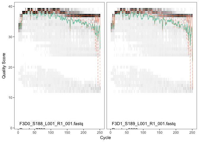
The forward reads are good quality. We generally advise trimming the last few nucleotides to avoid less well-controlled errors that can arise there. There is no suggestion from these quality profiles that any additional trimming is needed, so we will truncate the forward reads at position 240 (trimming the last 10 nucleotides).
Now we visualize the quality profile of the reverse reads:
1
    plotQualityProfile(fnRs[1:2])
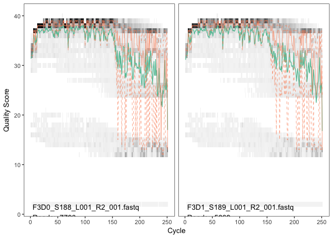 The
reverse reads are significantly worse quality, especially at the end,
which is common in Illumina sequencing. This isn’t too worrisome, DADA2
incorporates quality information into its error model which makes the
algorithm robust to lower quality sequence, but trimming as the average
qualities crash is still a good idea as long as our reads will still
overlap. We will truncate at position 160 where the quality distribution
crashes.
The
reverse reads are significantly worse quality, especially at the end,
which is common in Illumina sequencing. This isn’t too worrisome, DADA2
incorporates quality information into its error model which makes the
algorithm robust to lower quality sequence, but trimming as the average
qualities crash is still a good idea as long as our reads will still
overlap. We will truncate at position 160 where the quality distribution
crashes.
If using this workflow on your own data: Your reads must overlap after truncation in order to merge them later!!! The tutorial is using 2x250 V4 sequence data, so the forward and reverse reads almost completely overlap and our trimming can be completely guided by the quality scores. If you are using a less-overlapping primer set, like V1-V2 or V3-V4, your truncLen must be large enough to maintain the overlap between them (the more the better).
Perform filtering and trimming
We define the filenames for the filtered fastq.gz files:
1
2
3
    filt_path <- file.path(path, "filtered") # Place filtered files in filtered/ subdirectory
    filtFs <- file.path(filt_path, paste0(sample.names, "_F_filt.fastq.gz"))
    filtRs <- file.path(filt_path, paste0(sample.names, "_R_filt.fastq.gz"))
We’ll use standard filtering parameters: maxN=0 (DADA2 requires no Ns), truncQ=2, rm.phix=TRUE and maxEE=2. The maxEE parameter sets the maximum number of “expected errors” allowed in a read, which is a better filter than simply averaging quality scores.
Filter the forward and reverse reads:
1
2
3
4
5
6
7
8
9
10
11
12
    out <- filterAndTrim(fnFs, filtFs, fnRs, filtRs, truncLen=c(240,160),
                  maxN=0, maxEE=c(2,2), truncQ=2, rm.phix=TRUE,
                  compress=TRUE, multithread=TRUE)
    head(out)

    ##                               reads.in reads.out
    ## F3D0_S188_L001_R1_001.fastq       7793      7113
    ## F3D1_S189_L001_R1_001.fastq       5869      5299
    ## F3D141_S207_L001_R1_001.fastq     5958      5463
    ## F3D142_S208_L001_R1_001.fastq     3183      2914
    ## F3D143_S209_L001_R1_001.fastq     3178      2941
    ## F3D144_S210_L001_R1_001.fastq     4827      4312
If using this workflow on your own data: The standard filtering parameters are starting points, not set in stone. For example, if too few reads are passing the filter, considering relaxing maxEE, perhaps especially on the reverse reads (eg. maxEE=c(2,5)). If you want to speed up downstream computation, consider tightening maxEE. For pair-end reads consider the length of your amplicon when choosing truncLen as your reads must overlap after truncation in order to merge them later!!!
If using this workflow on your own data: For common ITS amplicon strategies, it is undesirable to truncate reads to a fixed length due to the large amount of length variation at that locus. That is OK, just leave out truncLen. Make sure you removed the forward and reverse primers from both the forward and reverse reads though!
# Learn the Error Rates The DADA2 algorithm depends on a parametric error model (err) and every amplicon dataset has a different set of error rates. The learnErrors method learns the error model from the data, by alternating estimation of the error rates and inference of sample composition until they converge on a jointly consistent solution. As in many optimization problems, the algorithm must begin with an initial guess, for which the maximum possible error rates in this data are used (the error rates if only the most abundant sequence is correct and all the rest are errors).
The following runs in about 1.5 minutes on a 2016 Macbook Pro:
1
2
3
4
5
6
7
8
9
10
11
12
13
14
15
16
17
18
19
20
21
22
23
24
25
26
27
28
29
30
31
32
33
34
35
    # Learn error rates, and time the procedure
    system.time(errF <- learnErrors(filtFs, multithread=TRUE))

    ## Initializing error rates to maximum possible estimate.
    ## Sample 1 - 7113 reads in 1979 unique sequences.
    ## Sample 2 - 5299 reads in 1639 unique sequences.
    ## Sample 3 - 5463 reads in 1477 unique sequences.
    ## Sample 4 - 2914 reads in 904 unique sequences.
    ## Sample 5 - 2941 reads in 939 unique sequences.
    ## Sample 6 - 4312 reads in 1267 unique sequences.
    ## Sample 7 - 6741 reads in 1756 unique sequences.
    ## Sample 8 - 4560 reads in 1438 unique sequences.
    ## Sample 9 - 15637 reads in 3590 unique sequences.
    ## Sample 10 - 11413 reads in 2762 unique sequences.
    ## Sample 11 - 12017 reads in 3021 unique sequences.
    ## Sample 12 - 5032 reads in 1566 unique sequences.
    ## Sample 13 - 18075 reads in 3707 unique sequences.
    ## Sample 14 - 6250 reads in 1479 unique sequences.
    ## Sample 15 - 4052 reads in 1195 unique sequences.
    ## Sample 16 - 7369 reads in 1832 unique sequences.
    ## Sample 17 - 4765 reads in 1183 unique sequences.
    ## Sample 18 - 4871 reads in 1382 unique sequences.
    ## Sample 19 - 6504 reads in 1709 unique sequences.
    ## Sample 20 - 4314 reads in 897 unique sequences.
    ##    selfConsist step 2
    ##    selfConsist step 3
    ##    selfConsist step 4
    ##    selfConsist step 5
    ##
    ##
    ## Convergence after  5  rounds.
    ## Total reads used:  139642

    ##    user  system elapsed
    ## 197.896   4.869  78.152
1
2
3
4
5
6
7
8
9
10
11
12
13
14
15
16
17
18
19
20
21
22
23
24
25
26
27
28
29
30
31
32
33
34
35
36
    # Learn error rates, time the procedure
    system.time(errR <- learnErrors(filtRs, multithread=TRUE))

    ## Initializing error rates to maximum possible estimate.
    ## Sample 1 - 7113 reads in 1660 unique sequences.
    ## Sample 2 - 5299 reads in 1349 unique sequences.
    ## Sample 3 - 5463 reads in 1335 unique sequences.
    ## Sample 4 - 2914 reads in 853 unique sequences.
    ## Sample 5 - 2941 reads in 880 unique sequences.
    ## Sample 6 - 4312 reads in 1286 unique sequences.
    ## Sample 7 - 6741 reads in 1803 unique sequences.
    ## Sample 8 - 4560 reads in 1265 unique sequences.
    ## Sample 9 - 15637 reads in 3414 unique sequences.
    ## Sample 10 - 11413 reads in 2522 unique sequences.
    ## Sample 11 - 12017 reads in 2771 unique sequences.
    ## Sample 12 - 5032 reads in 1415 unique sequences.
    ## Sample 13 - 18075 reads in 3290 unique sequences.
    ## Sample 14 - 6250 reads in 1390 unique sequences.
    ## Sample 15 - 4052 reads in 1134 unique sequences.
    ## Sample 16 - 7369 reads in 1635 unique sequences.
    ## Sample 17 - 4765 reads in 1084 unique sequences.
    ## Sample 18 - 4871 reads in 1161 unique sequences.
    ## Sample 19 - 6504 reads in 1502 unique sequences.
    ## Sample 20 - 4314 reads in 732 unique sequences.
    ##    selfConsist step 2
    ##    selfConsist step 3
    ##    selfConsist step 4
    ##    selfConsist step 5
    ##    selfConsist step 6
    ##
    ##
    ## Convergence after  6  rounds.
    ## Total reads used:  139642

    ##    user  system elapsed
    ## 150.270   3.872  60.280
It is always worthwhile, as a sanity check if nothing else, to visualize the estimated error rates:
1
2
3
4
5
    plotErrors(errF, nominalQ=TRUE)

    ## Warning: Transformation introduced infinite values in continuous y-axis

    ## Warning: Transformation introduced infinite values in continuous y-axis
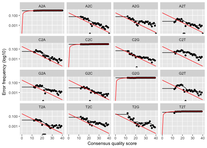 The
error rates for each possible transition (eg. A->C, A->G, …) are
shown. Points are the observed error rates for each consensus quality
score. The black line shows the estimated error rates after convergence.
The red line shows the error rates expected under the nominal definition
of the Q-value. Here the black line (the estimated rates) fits the
observed rates well, and the error rates drop with increased quality as
expected. Everything looks reasonable and we proceed with confidence.
The
error rates for each possible transition (eg. A->C, A->G, …) are
shown. Points are the observed error rates for each consensus quality
score. The black line shows the estimated error rates after convergence.
The red line shows the error rates expected under the nominal definition
of the Q-value. Here the black line (the estimated rates) fits the
observed rates well, and the error rates drop with increased quality as
expected. Everything looks reasonable and we proceed with confidence.
If using this workflow on your own data: Parameter learning is computationally intensive, so by default the learnErrors function uses only a subset of the data (the first 1M reads). If the plotted error model does not look like a good fit, try increasing the nreads parameter to see if the fit improves.
Dereplication
Dereplication combines all identical sequencing reads into into “unique sequences” with a corresponding “abundance”: the number of reads with that unique sequence. Dereplication substantially reduces computation time by eliminating redundant comparisons.
Dereplication in the DADA2 pipeline has one crucial addition from other pipelines: DADA2 retains a summary of the quality information associated with each unique sequence. The consensus quality profile of a unique sequence is the average of the positional qualities from the dereplicated reads. These quality profiles inform the error model of the subsequent denoising step, significantly increasing DADA2’s accuracy.
Dereplicate the filtered fastq files:
1
2
3
4
5
6
7
8
9
10
11
12
13
14
15
16
17
18
19
20
21
22
23
24
25
26
27
28
29
30
31
32
33
34
35
36
37
38
39
40
41
42
43
44
45
46
47
48
49
50
51
52
53
54
55
56
57
58
59
60
61
62
63
64
65
66
67
68
69
70
71
72
73
74
75
76
77
78
79
80
81
82
83
84
85
86
87
88
89
90
91
92
93
94
95
96
97
98
99
100
101
102
103
104
105
106
107
108
109
110
111
112
113
114
115
116
117
118
119
120
121
122
123
124
125
126
127
128
129
130
131
132
133
134
135
136
137
138
139
140
141
142
143
144
145
146
147
148
149
150
151
152
153
154
155
156
157
158
159
160
161
162
163
164
165
166
167
    derepFs <- derepFastq(filtFs, verbose=TRUE)

    ## Dereplicating sequence entries in Fastq file: /Users/rivers/Documents/MicrobiomeWorkshop/Amplicon_tutorial/MiSeq_SOP/filtered/F3D0_F_filt.fastq.gz

    ## Encountered 1979 unique sequences from 7113 total sequences read.

    ## Dereplicating sequence entries in Fastq file: /Users/rivers/Documents/MicrobiomeWorkshop/Amplicon_tutorial/MiSeq_SOP/filtered/F3D1_F_filt.fastq.gz

    ## Encountered 1639 unique sequences from 5299 total sequences read.

    ## Dereplicating sequence entries in Fastq file: /Users/rivers/Documents/MicrobiomeWorkshop/Amplicon_tutorial/MiSeq_SOP/filtered/F3D141_F_filt.fastq.gz

    ## Encountered 1477 unique sequences from 5463 total sequences read.

    ## Dereplicating sequence entries in Fastq file: /Users/rivers/Documents/MicrobiomeWorkshop/Amplicon_tutorial/MiSeq_SOP/filtered/F3D142_F_filt.fastq.gz

    ## Encountered 904 unique sequences from 2914 total sequences read.

    ## Dereplicating sequence entries in Fastq file: /Users/rivers/Documents/MicrobiomeWorkshop/Amplicon_tutorial/MiSeq_SOP/filtered/F3D143_F_filt.fastq.gz

    ## Encountered 939 unique sequences from 2941 total sequences read.

    ## Dereplicating sequence entries in Fastq file: /Users/rivers/Documents/MicrobiomeWorkshop/Amplicon_tutorial/MiSeq_SOP/filtered/F3D144_F_filt.fastq.gz

    ## Encountered 1267 unique sequences from 4312 total sequences read.

    ## Dereplicating sequence entries in Fastq file: /Users/rivers/Documents/MicrobiomeWorkshop/Amplicon_tutorial/MiSeq_SOP/filtered/F3D145_F_filt.fastq.gz

    ## Encountered 1756 unique sequences from 6741 total sequences read.

    ## Dereplicating sequence entries in Fastq file: /Users/rivers/Documents/MicrobiomeWorkshop/Amplicon_tutorial/MiSeq_SOP/filtered/F3D146_F_filt.fastq.gz

    ## Encountered 1438 unique sequences from 4560 total sequences read.

    ## Dereplicating sequence entries in Fastq file: /Users/rivers/Documents/MicrobiomeWorkshop/Amplicon_tutorial/MiSeq_SOP/filtered/F3D147_F_filt.fastq.gz

    ## Encountered 3590 unique sequences from 15637 total sequences read.

    ## Dereplicating sequence entries in Fastq file: /Users/rivers/Documents/MicrobiomeWorkshop/Amplicon_tutorial/MiSeq_SOP/filtered/F3D148_F_filt.fastq.gz

    ## Encountered 2762 unique sequences from 11413 total sequences read.

    ## Dereplicating sequence entries in Fastq file: /Users/rivers/Documents/MicrobiomeWorkshop/Amplicon_tutorial/MiSeq_SOP/filtered/F3D149_F_filt.fastq.gz

    ## Encountered 3021 unique sequences from 12017 total sequences read.

    ## Dereplicating sequence entries in Fastq file: /Users/rivers/Documents/MicrobiomeWorkshop/Amplicon_tutorial/MiSeq_SOP/filtered/F3D150_F_filt.fastq.gz

    ## Encountered 1566 unique sequences from 5032 total sequences read.

    ## Dereplicating sequence entries in Fastq file: /Users/rivers/Documents/MicrobiomeWorkshop/Amplicon_tutorial/MiSeq_SOP/filtered/F3D2_F_filt.fastq.gz

    ## Encountered 3707 unique sequences from 18075 total sequences read.

    ## Dereplicating sequence entries in Fastq file: /Users/rivers/Documents/MicrobiomeWorkshop/Amplicon_tutorial/MiSeq_SOP/filtered/F3D3_F_filt.fastq.gz

    ## Encountered 1479 unique sequences from 6250 total sequences read.

    ## Dereplicating sequence entries in Fastq file: /Users/rivers/Documents/MicrobiomeWorkshop/Amplicon_tutorial/MiSeq_SOP/filtered/F3D5_F_filt.fastq.gz

    ## Encountered 1195 unique sequences from 4052 total sequences read.

    ## Dereplicating sequence entries in Fastq file: /Users/rivers/Documents/MicrobiomeWorkshop/Amplicon_tutorial/MiSeq_SOP/filtered/F3D6_F_filt.fastq.gz

    ## Encountered 1832 unique sequences from 7369 total sequences read.

    ## Dereplicating sequence entries in Fastq file: /Users/rivers/Documents/MicrobiomeWorkshop/Amplicon_tutorial/MiSeq_SOP/filtered/F3D7_F_filt.fastq.gz

    ## Encountered 1183 unique sequences from 4765 total sequences read.

    ## Dereplicating sequence entries in Fastq file: /Users/rivers/Documents/MicrobiomeWorkshop/Amplicon_tutorial/MiSeq_SOP/filtered/F3D8_F_filt.fastq.gz

    ## Encountered 1382 unique sequences from 4871 total sequences read.

    ## Dereplicating sequence entries in Fastq file: /Users/rivers/Documents/MicrobiomeWorkshop/Amplicon_tutorial/MiSeq_SOP/filtered/F3D9_F_filt.fastq.gz

    ## Encountered 1709 unique sequences from 6504 total sequences read.

    ## Dereplicating sequence entries in Fastq file: /Users/rivers/Documents/MicrobiomeWorkshop/Amplicon_tutorial/MiSeq_SOP/filtered/Mock_F_filt.fastq.gz

    ## Encountered 897 unique sequences from 4314 total sequences read.

    derepRs <- derepFastq(filtRs, verbose=TRUE)

    ## Dereplicating sequence entries in Fastq file: /Users/rivers/Documents/MicrobiomeWorkshop/Amplicon_tutorial/MiSeq_SOP/filtered/F3D0_R_filt.fastq.gz

    ## Encountered 1660 unique sequences from 7113 total sequences read.

    ## Dereplicating sequence entries in Fastq file: /Users/rivers/Documents/MicrobiomeWorkshop/Amplicon_tutorial/MiSeq_SOP/filtered/F3D1_R_filt.fastq.gz

    ## Encountered 1349 unique sequences from 5299 total sequences read.

    ## Dereplicating sequence entries in Fastq file: /Users/rivers/Documents/MicrobiomeWorkshop/Amplicon_tutorial/MiSeq_SOP/filtered/F3D141_R_filt.fastq.gz

    ## Encountered 1335 unique sequences from 5463 total sequences read.

    ## Dereplicating sequence entries in Fastq file: /Users/rivers/Documents/MicrobiomeWorkshop/Amplicon_tutorial/MiSeq_SOP/filtered/F3D142_R_filt.fastq.gz

    ## Encountered 853 unique sequences from 2914 total sequences read.

    ## Dereplicating sequence entries in Fastq file: /Users/rivers/Documents/MicrobiomeWorkshop/Amplicon_tutorial/MiSeq_SOP/filtered/F3D143_R_filt.fastq.gz

    ## Encountered 880 unique sequences from 2941 total sequences read.

    ## Dereplicating sequence entries in Fastq file: /Users/rivers/Documents/MicrobiomeWorkshop/Amplicon_tutorial/MiSeq_SOP/filtered/F3D144_R_filt.fastq.gz

    ## Encountered 1286 unique sequences from 4312 total sequences read.

    ## Dereplicating sequence entries in Fastq file: /Users/rivers/Documents/MicrobiomeWorkshop/Amplicon_tutorial/MiSeq_SOP/filtered/F3D145_R_filt.fastq.gz

    ## Encountered 1803 unique sequences from 6741 total sequences read.

    ## Dereplicating sequence entries in Fastq file: /Users/rivers/Documents/MicrobiomeWorkshop/Amplicon_tutorial/MiSeq_SOP/filtered/F3D146_R_filt.fastq.gz

    ## Encountered 1265 unique sequences from 4560 total sequences read.

    ## Dereplicating sequence entries in Fastq file: /Users/rivers/Documents/MicrobiomeWorkshop/Amplicon_tutorial/MiSeq_SOP/filtered/F3D147_R_filt.fastq.gz

    ## Encountered 3414 unique sequences from 15637 total sequences read.

    ## Dereplicating sequence entries in Fastq file: /Users/rivers/Documents/MicrobiomeWorkshop/Amplicon_tutorial/MiSeq_SOP/filtered/F3D148_R_filt.fastq.gz

    ## Encountered 2522 unique sequences from 11413 total sequences read.

    ## Dereplicating sequence entries in Fastq file: /Users/rivers/Documents/MicrobiomeWorkshop/Amplicon_tutorial/MiSeq_SOP/filtered/F3D149_R_filt.fastq.gz

    ## Encountered 2771 unique sequences from 12017 total sequences read.

    ## Dereplicating sequence entries in Fastq file: /Users/rivers/Documents/MicrobiomeWorkshop/Amplicon_tutorial/MiSeq_SOP/filtered/F3D150_R_filt.fastq.gz

    ## Encountered 1415 unique sequences from 5032 total sequences read.

    ## Dereplicating sequence entries in Fastq file: /Users/rivers/Documents/MicrobiomeWorkshop/Amplicon_tutorial/MiSeq_SOP/filtered/F3D2_R_filt.fastq.gz

    ## Encountered 3290 unique sequences from 18075 total sequences read.

    ## Dereplicating sequence entries in Fastq file: /Users/rivers/Documents/MicrobiomeWorkshop/Amplicon_tutorial/MiSeq_SOP/filtered/F3D3_R_filt.fastq.gz

    ## Encountered 1390 unique sequences from 6250 total sequences read.

    ## Dereplicating sequence entries in Fastq file: /Users/rivers/Documents/MicrobiomeWorkshop/Amplicon_tutorial/MiSeq_SOP/filtered/F3D5_R_filt.fastq.gz

    ## Encountered 1134 unique sequences from 4052 total sequences read.

    ## Dereplicating sequence entries in Fastq file: /Users/rivers/Documents/MicrobiomeWorkshop/Amplicon_tutorial/MiSeq_SOP/filtered/F3D6_R_filt.fastq.gz

    ## Encountered 1635 unique sequences from 7369 total sequences read.

    ## Dereplicating sequence entries in Fastq file: /Users/rivers/Documents/MicrobiomeWorkshop/Amplicon_tutorial/MiSeq_SOP/filtered/F3D7_R_filt.fastq.gz

    ## Encountered 1084 unique sequences from 4765 total sequences read.

    ## Dereplicating sequence entries in Fastq file: /Users/rivers/Documents/MicrobiomeWorkshop/Amplicon_tutorial/MiSeq_SOP/filtered/F3D8_R_filt.fastq.gz

    ## Encountered 1161 unique sequences from 4871 total sequences read.

    ## Dereplicating sequence entries in Fastq file: /Users/rivers/Documents/MicrobiomeWorkshop/Amplicon_tutorial/MiSeq_SOP/filtered/F3D9_R_filt.fastq.gz

    ## Encountered 1502 unique sequences from 6504 total sequences read.

    ## Dereplicating sequence entries in Fastq file: /Users/rivers/Documents/MicrobiomeWorkshop/Amplicon_tutorial/MiSeq_SOP/filtered/Mock_R_filt.fastq.gz

    ## Encountered 732 unique sequences from 4314 total sequences read.

    # Name the derep-class objects by the sample names
    names(derepFs) <- sample.names
    names(derepRs) <- sample.names
If using this workflow on your own data: The tutorial dataset is small enough to easily load into memory. If your dataset exceeds available RAM, it is preferable to process samples one-by-one in a streaming fashion: see the DADA2 Workflow on Big Data for an example.
Sample Inference
We are now ready to apply the core sequence-variant inference algorithm to the dereplicated data.
Infer the sequence variants in each sample:
1
2
3
4
5
6
7
8
9
10
11
12
13
14
15
16
17
18
19
20
21
22
23
24
25
    system.time(dadaFs <- dada(derepFs, err=errF, multithread=TRUE))

    ## Sample 1 - 7113 reads in 1979 unique sequences.
    ## Sample 2 - 5299 reads in 1639 unique sequences.
    ## Sample 3 - 5463 reads in 1477 unique sequences.
    ## Sample 4 - 2914 reads in 904 unique sequences.
    ## Sample 5 - 2941 reads in 939 unique sequences.
    ## Sample 6 - 4312 reads in 1267 unique sequences.
    ## Sample 7 - 6741 reads in 1756 unique sequences.
    ## Sample 8 - 4560 reads in 1438 unique sequences.
    ## Sample 9 - 15637 reads in 3590 unique sequences.
    ## Sample 10 - 11413 reads in 2762 unique sequences.
    ## Sample 11 - 12017 reads in 3021 unique sequences.
    ## Sample 12 - 5032 reads in 1566 unique sequences.
    ## Sample 13 - 18075 reads in 3707 unique sequences.
    ## Sample 14 - 6250 reads in 1479 unique sequences.
    ## Sample 15 - 4052 reads in 1195 unique sequences.
    ## Sample 16 - 7369 reads in 1832 unique sequences.
    ## Sample 17 - 4765 reads in 1183 unique sequences.
    ## Sample 18 - 4871 reads in 1382 unique sequences.
    ## Sample 19 - 6504 reads in 1709 unique sequences.
    ## Sample 20 - 4314 reads in 897 unique sequences.

    ##    user  system elapsed
    ##  42.754   1.012  16.803
1
2
3
4
5
6
7
8
9
10
11
12
13
14
15
16
17
18
19
20
21
22
    dadaRs <- dada(derepRs, err=errR, multithread=TRUE)

    ## Sample 1 - 7113 reads in 1660 unique sequences.
    ## Sample 2 - 5299 reads in 1349 unique sequences.
    ## Sample 3 - 5463 reads in 1335 unique sequences.
    ## Sample 4 - 2914 reads in 853 unique sequences.
    ## Sample 5 - 2941 reads in 880 unique sequences.
    ## Sample 6 - 4312 reads in 1286 unique sequences.
    ## Sample 7 - 6741 reads in 1803 unique sequences.
    ## Sample 8 - 4560 reads in 1265 unique sequences.
    ## Sample 9 - 15637 reads in 3414 unique sequences.
    ## Sample 10 - 11413 reads in 2522 unique sequences.
    ## Sample 11 - 12017 reads in 2771 unique sequences.
    ## Sample 12 - 5032 reads in 1415 unique sequences.
    ## Sample 13 - 18075 reads in 3290 unique sequences.
    ## Sample 14 - 6250 reads in 1390 unique sequences.
    ## Sample 15 - 4052 reads in 1134 unique sequences.
    ## Sample 16 - 7369 reads in 1635 unique sequences.
    ## Sample 17 - 4765 reads in 1084 unique sequences.
    ## Sample 18 - 4871 reads in 1161 unique sequences.
    ## Sample 19 - 6504 reads in 1502 unique sequences.
    ## Sample 20 - 4314 reads in 732 unique sequences.
Inspecting the dada-class object returned by dada:
1
2
3
4
5
    dadaFs[[1]]

    ## dada-class: object describing DADA2 denoising results
    ## 128 sample sequences were inferred from 1979 input unique sequences.
    ## Key parameters: OMEGA_A = 1e-40, BAND_SIZE = 16, USE_QUALS = TRUE
The DADA2 algorithm inferred 128 real variants from the 1979 unique sequences in the first sample. There is much more to the dada-class return object than this (see help(“dada-class”) for some info), including multiple diagnostics about the quality of each inferred sequence variant, but that is beyond the scope of an introductory tutorial.
If using this workflow on your own data: All samples are simultaneously loaded into memory in the tutorial. If you are dealing with datasets that approach or exceed available RAM, it is preferable to process samples one-by-one in a streaming fashion: see the DADA2 Workflow on Big Data for an example.
If using this workflow on your own data: By default, the dada function processes each sample independently, but pooled processing is available with pool=TRUE and that may give better results for low sampling depths at the cost of increased computation time. See our discussion about pooling samples for sample inference.
Merge paired reads
Spurious sequence variants are further reduced by merging overlapping reads. The core function here is mergePairs, which depends on the forward and reverse reads being in matching order at the time they were dereplicated.
Merge the denoised forward and reverse reads:
1
2
3
4
5
6
7
8
9
10
11
12
13
14
15
16
17
18
19
20
21
22
23
24
25
26
27
28
29
30
31
32
33
34
35
36
37
38
39
40
41
42
43
44
45
46
47
48
49
50
51
52
53
54
55
56
57
58
59
    mergers <- mergePairs(dadaFs, derepFs, dadaRs, derepRs, verbose=TRUE)

    ## 6600 paired-reads (in 105 unique pairings) successfully merged out of 7113 (in 254 pairings) input.

    ## 5078 paired-reads (in 100 unique pairings) successfully merged out of 5299 (in 192 pairings) input.

    ## 5047 paired-reads (in 78 unique pairings) successfully merged out of 5463 (in 199 pairings) input.

    ## 2663 paired-reads (in 52 unique pairings) successfully merged out of 2914 (in 142 pairings) input.

    ## 2575 paired-reads (in 54 unique pairings) successfully merged out of 2941 (in 162 pairings) input.

    ## 3668 paired-reads (in 53 unique pairings) successfully merged out of 4312 (in 203 pairings) input.

    ## 6202 paired-reads (in 81 unique pairings) successfully merged out of 6741 (in 230 pairings) input.

    ## 4040 paired-reads (in 90 unique pairings) successfully merged out of 4560 (in 233 pairings) input.

    ## 14340 paired-reads (in 142 unique pairings) successfully merged out of 15637 (in 410 pairings) input.

    ## 10599 paired-reads (in 117 unique pairings) successfully merged out of 11413 (in 331 pairings) input.

    ## 11197 paired-reads (in 134 unique pairings) successfully merged out of 12017 (in 342 pairings) input.

    ## 4426 paired-reads (in 83 unique pairings) successfully merged out of 5032 (in 233 pairings) input.

    ## 17477 paired-reads (in 148 unique pairings) successfully merged out of 18075 (in 330 pairings) input.

    ## 5907 paired-reads (in 80 unique pairings) successfully merged out of 6250 (in 193 pairings) input.

    ## 3770 paired-reads (in 85 unique pairings) successfully merged out of 4052 (in 194 pairings) input.

    ## 6915 paired-reads (in 98 unique pairings) successfully merged out of 7369 (in 226 pairings) input.

    ## 4480 paired-reads (in 66 unique pairings) successfully merged out of 4765 (in 159 pairings) input.

    ## 4606 paired-reads (in 96 unique pairings) successfully merged out of 4871 (in 204 pairings) input.

    ## 6173 paired-reads (in 108 unique pairings) successfully merged out of 6504 (in 196 pairings) input.

    ## 4279 paired-reads (in 20 unique pairings) successfully merged out of 4314 (in 33 pairings) input.

    # Inspect the merger data.frame from the first sample
    head(mergers[[1]])

    ##                                                                                                                                                                                                                                                       sequence
    ## 1 TACGGAGGATGCGAGCGTTATCCGGATTTATTGGGTTTAAAGGGTGCGCAGGCGGAAGATCAAGTCAGCGGTAAAATTGAGAGGCTCAACCTCTTCGAGCCGTTGAAACTGGTTTTCTTGAGTGAGCGAGAAGTATGCGGAATGCGTGGTGTAGCGGTGAAATGCATAGATATCACGCAGAACTCCGATTGCGAAGGCAGCATACCGGCGCTCAACTGACGCTCATGCACGAAAGTGTGGGTATCGAACAGG
    ## 2 TACGGAGGATGCGAGCGTTATCCGGATTTATTGGGTTTAAAGGGTGCGTAGGCGGCCTGCCAAGTCAGCGGTAAAATTGCGGGGCTCAACCCCGTACAGCCGTTGAAACTGCCGGGCTCGAGTGGGCGAGAAGTATGCGGAATGCGTGGTGTAGCGGTGAAATGCATAGATATCACGCAGAACCCCGATTGCGAAGGCAGCATACCGGCGCCCTACTGACGCTGAGGCACGAAAGTGCGGGGATCAAACAGG
    ## 3 TACGGAGGATGCGAGCGTTATCCGGATTTATTGGGTTTAAAGGGTGCGTAGGCGGGCTGTTAAGTCAGCGGTCAAATGTCGGGGCTCAACCCCGGCCTGCCGTTGAAACTGGCGGCCTCGAGTGGGCGAGAAGTATGCGGAATGCGTGGTGTAGCGGTGAAATGCATAGATATCACGCAGAACTCCGATTGCGAAGGCAGCATACCGGCGCCCGACTGACGCTGAGGCACGAAAGCGTGGGTATCGAACAGG
    ## 4 TACGGAGGATGCGAGCGTTATCCGGATTTATTGGGTTTAAAGGGTGCGTAGGCGGGCTTTTAAGTCAGCGGTAAAAATTCGGGGCTCAACCCCGTCCGGCCGTTGAAACTGGGGGCCTTGAGTGGGCGAGAAGAAGGCGGAATGCGTGGTGTAGCGGTGAAATGCATAGATATCACGCAGAACCCCGATTGCGAAGGCAGCCTTCCGGCGCCCTACTGACGCTGAGGCACGAAAGTGCGGGGATCGAACAGG
    ## 5 TACGGAGGATGCGAGCGTTATCCGGATTTATTGGGTTTAAAGGGTGCGCAGGCGGACTCTCAAGTCAGCGGTCAAATCGCGGGGCTCAACCCCGTTCCGCCGTTGAAACTGGGAGCCTTGAGTGCGCGAGAAGTAGGCGGAATGCGTGGTGTAGCGGTGAAATGCATAGATATCACGCAGAACTCCGATTGCGAAGGCAGCCTACCGGCGCGCAACTGACGCTCATGCACGAAAGCGTGGGTATCGAACAGG
    ## 6 TACGGAGGATGCGAGCGTTATCCGGATTTATTGGGTTTAAAGGGTGCGTAGGCGGGATGCCAAGTCAGCGGTAAAAAAGCGGTGCTCAACGCCGTCGAGCCGTTGAAACTGGCGTTCTTGAGTGGGCGAGAAGTATGCGGAATGCGTGGTGTAGCGGTGAAATGCATAGATATCACGCAGAACTCCGATTGCGAAGGCAGCATACCGGCGCCCTACTGACGCTGAGGCACGAAAGCGTGGGTATCGAACAGG
    ##   abundance forward reverse nmatch nmismatch nindel prefer accept
    ## 1       586       1       1    148         0      0      1   TRUE
    ## 2       471       2       2    148         0      0      2   TRUE
    ## 3       451       3       4    148         0      0      1   TRUE
    ## 4       433       4       3    148         0      0      2   TRUE
    ## 5       353       5       6    148         0      0      1   TRUE
    ## 6       285       6       5    148         0      0      2   TRUE
We now have a data.frame for each sample with the merged $sequence, its $abundance, and the indices of the merged $forward and $reverse denoised sequences. Paired reads that did not exactly overlap were removed by mergePairs.
If using this workflow on your own data: Most of your reads should successfully merge. If that is not the case upstream parameters may need to be revisited: Did you trim away the overlap between your reads?
Construct sequence table We can now construct a “sequence table” of our mouse samples, a higher-resolution version of the “OTU table” produced by classical methods:
1
2
3
4
5
6
7
8
9
10
11
12
13
14
15
16
    seqtab <- makeSequenceTable(mergers)

    ## The sequences being tabled vary in length.

    dim(seqtab)

    ## [1]  20 288

    # Inspect distribution of sequence lengths
    table(nchar(getSequences(seqtab)))

    ##
    ## 251 252 253 254 255
    ##   1  87 192   6   2

    hist(nchar(getSequences(seqtab)), main="Distribution of sequence lengths")
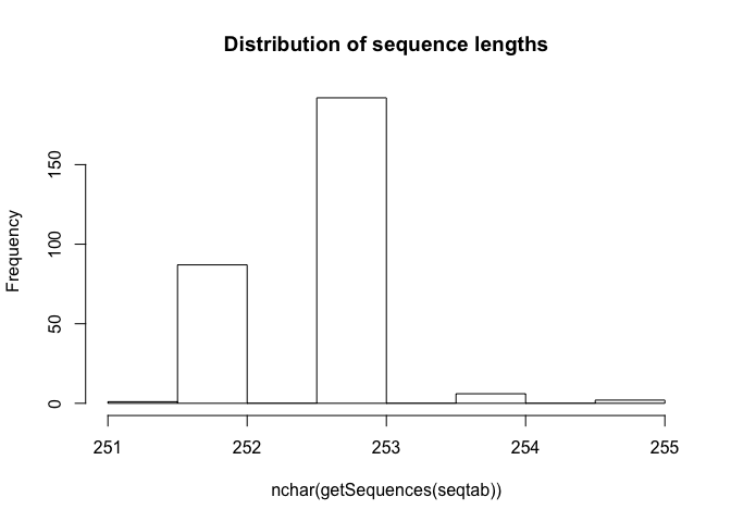 The
sequence table is a matrix with rows corresponding to (and named by) the
samples, and columns corresponding to (and named by) the sequence
variants. The lengths of our merged sequences all fall within the
expected range for this V4 amplicon.
The
sequence table is a matrix with rows corresponding to (and named by) the
samples, and columns corresponding to (and named by) the sequence
variants. The lengths of our merged sequences all fall within the
expected range for this V4 amplicon.
If using this workflow on your own data: Sequences that are much longer or shorter than expected may be the result of non-specific priming, and may be worth removing (eg. seqtab2 <- seqtab[,nchar(colnames(seqtab)) %in% seq(250,256)]). This is analogous to “cutting a band” in-silico to get amplicons of the targeted length.
Remove chimeras
The core dada method removes substitution and indel errors, but chimeras remain. Fortunately, the accuracy of the sequences after denoising makes identifying chimeras simpler than it is when dealing with fuzzy OTUs: all sequences which can be exactly reconstructed as a bimera (two-parent chimera) from more abundant sequences.
1
2
3
4
5
6
7
8
9
10
11
    seqtab.nochim <- removeBimeraDenovo(seqtab, method="consensus", multithread=TRUE, verbose=TRUE)

    ## Identified 59 bimeras out of 288 input sequences.

    dim(seqtab.nochim)

    ## [1]  20 229

    sum(seqtab.nochim)/sum(seqtab)

    ## [1] 0.9643192
The fraction of chimeras varies based on factors including experimental procedures and sample complexity, but can be substantial. Here chimeras make up about 20% of the inferred sequence variants, but those variants account for only about 4% of the total sequence reads.
If using this workflow on your own data: Most of your reads should remain after chimera removal (it is not uncommon for a majority of sequence variants to be removed though). If most of your reads were removed as chimeric, upstream processing may need to be revisited. In almost all cases this is caused by primer sequences with ambiguous nucleotides that were not removed prior to beginning the DADA2 pipeline.
Track reads through the pipeline
As a final check of our progress, we’ll look at the number of reads that made it through each step in the pipeline:
1
2
3
4
5
6
7
8
9
10
11
12
13
    getN <- function(x) sum(getUniques(x))
    track <- cbind(out, sapply(dadaFs, getN), sapply(mergers, getN), rowSums(seqtab), rowSums(seqtab.nochim))
    colnames(track) <- c("input", "filtered", "denoised", "merged", "tabled", "nonchim")
    rownames(track) <- sample.names
    head(track)

    ##        input filtered denoised merged tabled nonchim
    ## F3D0    7793     7113     7113   6600   6600    6588
    ## F3D1    5869     5299     5299   5078   5078    5067
    ## F3D141  5958     5463     5463   5047   5047    4928
    ## F3D142  3183     2914     2914   2663   2663    2600
    ## F3D143  3178     2941     2941   2575   2575    2550
    ## F3D144  4827     4312     4312   3668   3668    3527
Looks good, we kept the majority of our raw reads, and there is no over-large drop associated with any single step.
If using this workflow on your own data: This is a great place to do a last sanity check. Outside of filtering (depending on how stringent you want to be) there should no step in which a majority of reads are lost. If a majority of reads failed to merge, you may need to revisit the truncLen parameter used in the filtering step and make sure that the truncated reads span your amplicon. If a majority of reads failed to pass the chimera check, you may need to revisit the removal of primers, as the ambiguous nucleotides in unremoved primers interfere with chimera identification.
Assign taxonomy
It is common at this point, especially in 16S/18S/ITS amplicon sequencing, to classify sequence variants taxonomically. The DADA2 package provides a native implementation of the RDP’s naive Bayesian classifier for this purpose. The assignTaxonomy function takes a set of sequences and a training set of taxonomically classified sequences, and outputs the taxonomic assignments with at least minBoot bootstrap confidence.
Appropriately formatted training fastas for the RDP training set 14, the GreenGenes 13.8 release clustered at 97% identity, the Silva reference database v123 (Silva dual license), and the UNITE ITS database (use the General Fasta release files) are available. To follow along, download the silva_nr_v123_train_set.fa.gz file, and place it in the directory with the fastq files.
The following databases are available:
Maintained:
- GreenGenes version 13.8
- RDP version 14
- Silva version 123 (Silva dual-license)
- UNITE (General Fasta releases) (version 1.3.3 or later of the dada2 package)
Contributed:
- HitDB version 1 (Human InTestinal 16S rRNA)
Note that currently species-assignment training fastas are only available for the Silva and RDP databases. In addition to thanking the folks at RDP, Silva and GreenGenes for making these datasets available, we also want to thank Pat Schloss and the mothur team for making cleaner versions of the Silva and RDP training set available. To be specific, we created the dada2-compatible training fastas from the mothur-compatible Silva.nr_v123 files (described here, and license here), the mothur-compatible 16S rRNA reference (RDP) (described here), and the GreenGenes 13.8 OTUs clustered at 97%.
Formatting custom databases
Custom databases can be used as well, provided they can be converted to the dada2-compatible training fasta format.
The assignTaxonomy(…) function expects the training data to be provided in the form of a fasta file (or compressed fasta file) in which the taxonomy corresponding to each sequence is encoded in the id line in the following fashion (the second sequence is not assigned down to level 6):
1
2
3
4
5
6
7
8
9
10
11
12
13
14
15
16
17
18
    taxtrain <- paste0(base_path,"silva_nr_v123_train_set.fa.gz")
    taxa <- assignTaxonomy(seqtab.nochim, taxtrain, multithread=TRUE)
    unname(head(taxa))

    ##      [,1]       [,2]            [,3]          [,4]
    ## [1,] "Bacteria" "Bacteroidetes" "Bacteroidia" "Bacteroidales"
    ## [2,] "Bacteria" "Bacteroidetes" "Bacteroidia" "Bacteroidales"
    ## [3,] "Bacteria" "Bacteroidetes" "Bacteroidia" "Bacteroidales"
    ## [4,] "Bacteria" "Bacteroidetes" "Bacteroidia" "Bacteroidales"
    ## [5,] "Bacteria" "Bacteroidetes" "Bacteroidia" "Bacteroidales"
    ## [6,] "Bacteria" "Bacteroidetes" "Bacteroidia" "Bacteroidales"
    ##      [,5]                        [,6]
    ## [1,] "Bacteroidales_S24-7_group" NA
    ## [2,] "Bacteroidales_S24-7_group" NA
    ## [3,] "Bacteroidales_S24-7_group" NA
    ## [4,] "Bacteroidales_S24-7_group" NA
    ## [5,] "Bacteroidaceae"            "Bacteroides"
    ## [6,] "Bacteroidales_S24-7_group" NA
Okay you’ve done it. You’ve sequenced, cleaned, clustered, removed chimeras and identified the microbial sequences in your sample. Now it’s time to begin making sense of that data.
Handoff to phyloseq
The DADA2 pipeline produced a sequence table and a taxonomy table which is appropriate for further analysis in phyloseq. We’ll also include the small amount of metadata we have – the samples are named by the gender (G), mouse subject number (X) and the day post-weaning (Y) it was sampled (eg. GXDY).
Import into phyloseq:
1
2
3
4
5
6
7
8
9
10
11
12
13
14
15
16
17
18
19
20
21
22
23
24
25
26
27
28
29
30
    library(phyloseq); packageVersion("phyloseq")

    ## [1] '1.20.0'

    library(ggplot2); packageVersion("ggplot2")

    ## [1] '2.2.1'

    # Make a data.frame holding the sample data
    samples.out <- rownames(seqtab.nochim)
    subject <- sapply(strsplit(samples.out, "D"), `[`, 1)
    gender <- substr(subject,1,1)
    subject <- substr(subject,2,999)
    day <- as.integer(sapply(strsplit(samples.out, "D"), `[`, 2))
    samdf <- data.frame(Subject=subject, Gender=gender, Day=day)
    samdf$When <- "Early"
    samdf$When[samdf$Day>100] <- "Late"
    rownames(samdf) <- samples.out

    # Construct phyloseq object (straightforward from dada2 outputs)
    ps <- phyloseq(otu_table(seqtab.nochim, taxa_are_rows=FALSE),
                   sample_data(samdf),
                   tax_table(taxa))
    ps <- prune_samples(sample_names(ps) != "Mock", ps) # Remove mock sample
    ps

    ## phyloseq-class experiment-level object
    ## otu_table()   OTU Table:         [ 229 taxa and 19 samples ]
    ## sample_data() Sample Data:       [ 19 samples by 4 sample variables ]
    ## tax_table()   Taxonomy Table:    [ 229 taxa by 6 taxonomic ranks ]
Plot the species richness =========================
1
2
3
4
5
6
7
8
    plot_richness(ps, x="Day", measures=c("Shannon", "Simpson"), color="When") + theme_bw()

    ## Warning in estimate_richness(physeq, split = TRUE, measures = measures): The data you have provided does not have
    ## any singletons. This is highly suspicious. Results of richness
    ## estimates (for example) are probably unreliable, or wrong, if you have already
    ## trimmed low-abundance taxa from the data.
    ##
    ## We recommended that you find the un-trimmed data and retry.
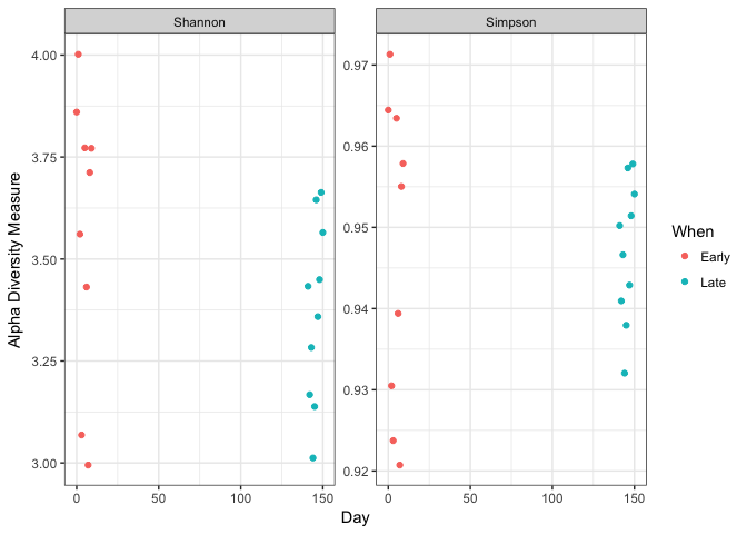
No obvious systematic difference in alpha-diversity between early and late samples.
Create ordination plots
1
2
3
4
5
6
7
8
9
10
11
12
13
14
15
16
17
18
19
20
21
22
23
24
25
26
27
28
29
30
31
32
33
34
35
36
37
38
39
40
41
42
43
44
45
46
47
48
49
50
51
    ord.nmds.bray <- ordinate(ps, method="NMDS", distance="bray")

    ## Square root transformation
    ## Wisconsin double standardization
    ## Run 0 stress 0.08908957
    ## Run 1 stress 0.1576644
    ## Run 2 stress 0.1534744
    ## Run 3 stress 0.08908957
    ## ... New best solution
    ## ... Procrustes: rmse 1.067254e-05  max resid 2.241028e-05
    ## ... Similar to previous best
    ## Run 4 stress 0.08908957
    ## ... Procrustes: rmse 4.473619e-06  max resid 1.027824e-05
    ## ... Similar to previous best
    ## Run 5 stress 0.08908957
    ## ... Procrustes: rmse 5.282251e-06  max resid 1.277511e-05
    ## ... Similar to previous best
    ## Run 6 stress 0.08908957
    ## ... Procrustes: rmse 1.159049e-05  max resid 2.817292e-05
    ## ... Similar to previous best
    ## Run 7 stress 0.09001158
    ## Run 8 stress 0.08908957
    ## ... Procrustes: rmse 1.767704e-05  max resid 4.100563e-05
    ## ... Similar to previous best
    ## Run 9 stress 0.08908957
    ## ... Procrustes: rmse 6.018521e-06  max resid 1.367387e-05
    ## ... Similar to previous best
    ## Run 10 stress 0.1558085
    ## Run 11 stress 0.1570124
    ## Run 12 stress 0.08908957
    ## ... Procrustes: rmse 1.571414e-05  max resid 3.483069e-05
    ## ... Similar to previous best
    ## Run 13 stress 0.1483247
    ## Run 14 stress 0.08908957
    ## ... Procrustes: rmse 1.05388e-05  max resid 2.781617e-05
    ## ... Similar to previous best
    ## Run 15 stress 0.09001142
    ## Run 16 stress 0.1572166
    ## Run 17 stress 0.08908966
    ## ... Procrustes: rmse 8.178829e-05  max resid 0.0001931953
    ## ... Similar to previous best
    ## Run 18 stress 0.08908957
    ## ... Procrustes: rmse 8.568774e-06  max resid 2.273861e-05
    ## ... Similar to previous best
    ## Run 19 stress 0.08908957
    ## ... Procrustes: rmse 9.447789e-06  max resid 2.287006e-05
    ## ... Similar to previous best
    ## Run 20 stress 0.09001141
    ## *** Solution reached

    plot_ordination(ps, ord.nmds.bray, color="When", title="Bray NMDS")
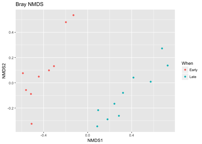 Ordination picks out a clear separation between the early and late
samples.
Ordination picks out a clear separation between the early and late
samples.
Bar plot
1
2
3
4
    top20 <- names(sort(taxa_sums(ps), decreasing=TRUE))[1:20]
    ps.top20 <- transform_sample_counts(ps, function(OTU) OTU/sum(OTU))
    ps.top20 <- prune_taxa(top20, ps.top20)
    plot_bar(ps.top20, x="Day", fill="Family") + facet_wrap(~When, scales="free_x")
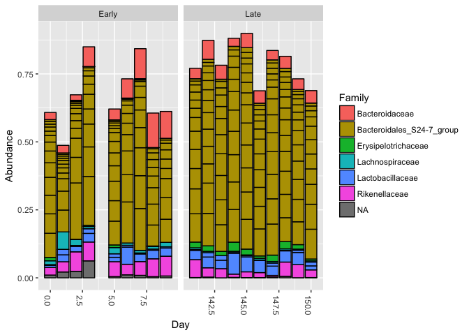
Nothing glaringly obvious jumps out from the taxonomic distribution of the top 20 sequences to explain the early-late differentiation.
Phylogenetic trees of amplicon sequences
It is common to create a phylogenetic tree of the taxa and then use metrics like UNIFRAC distance or just plot datain a phylogentic context.
That can be done in phyloseq too.
Align the sequences
1
2
3
4
5
6
7
8
9
10
11
12
13
14
15
16
17
18
19
20
21
22
23
24
25
26
27
28
29
30
31
32
33
34
35
36
37
38
39
40
41
42
43
44
45
46
47
48
49
50
51
52
53
54
55
56
57
58
59
60
61
62
63
64
65
    library("msa")

    ## Loading required package: Biostrings

    ## Loading required package: BiocGenerics

    ## Loading required package: parallel

    ##
    ## Attaching package: 'BiocGenerics'

    ## The following objects are masked from 'package:parallel':
    ##
    ##     clusterApply, clusterApplyLB, clusterCall, clusterEvalQ,
    ##     clusterExport, clusterMap, parApply, parCapply, parLapply,
    ##     parLapplyLB, parRapply, parSapply, parSapplyLB

    ## The following objects are masked from 'package:stats':
    ##
    ##     IQR, mad, sd, var, xtabs

    ## The following objects are masked from 'package:base':
    ##
    ##     anyDuplicated, append, as.data.frame, cbind, colMeans,
    ##     colnames, colSums, do.call, duplicated, eval, evalq, Filter,
    ##     Find, get, grep, grepl, intersect, is.unsorted, lapply,
    ##     lengths, Map, mapply, match, mget, order, paste, pmax,
    ##     pmax.int, pmin, pmin.int, Position, rank, rbind, Reduce,
    ##     rowMeans, rownames, rowSums, sapply, setdiff, sort, table,
    ##     tapply, union, unique, unsplit, which, which.max, which.min

    ## Loading required package: S4Vectors

    ## Loading required package: stats4

    ##
    ## Attaching package: 'S4Vectors'

    ## The following object is masked from 'package:base':
    ##
    ##     expand.grid

    ## Loading required package: IRanges

    ##
    ## Attaching package: 'IRanges'

    ## The following object is masked from 'package:phyloseq':
    ##
    ##     distance

    ## Loading required package: XVector

    ##
    ## Attaching package: 'Biostrings'

    ## The following object is masked from 'package:base':
    ##
    ##     strsplit

    seqs <- getSequences(seqtab.nochim)
    names(seqs) <- seqs # This propagates to the tip labels of the tree
    mult <- msa(seqs, method="ClustalW", type="dna", order="input")

    ## use default substitution matrix
TODO
- Make tree
- Calculate unifrac with the tree
- place data on tree see:
- https://bioconductor.org/packages/release/bioc/vignettes/phyloseq/inst/doc/phyloseq-analysis.html
- https://f1000research.com/articles/5-1492/v2
- DESEQ2
- SPIEC-EASI networks