ATAC-seq tutorial:
The data for this tutorial is based on this paper; Jégu et al., 2017. The authors describe the role of a chromatin remodeling protein in controlling Arabidopsis seedling morphogenesis by modulating chromatin accessibility. They base their conclusions on a combination of CHIPseq, ATAC-seq, MNAseseq and FAIREseq among other things. In this tutorial, we will work through the ATAC-seq dataset. Check the methods section in the paper for more details on the ATAC-seq library preparation, following the standard procedure.
1. Download fastq files directly from ENA website
The fastq files for all the experiments described are available at the ENA website under the bioproject PRJNA351855 The ATAC-seq data is the only paired end libraries in the list. We will visit the other files when talking about CHIPseq. We can download the reads directly using wget.
1
2
 wget ftp://ftp.sra.ebi.ac.uk/vol1/fastq/SRR473/002/SRR4733912/SRR4733912_1.fastq.gz
 wget ftp://ftp.sra.ebi.ac.uk/vol1/fastq/SRR473/002/SRR4733912/SRR4733912_2.fastq.gz
2. Quality Check
1
2
3
 mkdir Quality_ATAC
 module load fastqc
 fastqc -o Quality_ATAC /path/to/ATAC_paired/*.gz
We found that the nextera adapters have already been removed before depositing the sequences. We also confirmed this with the authors.
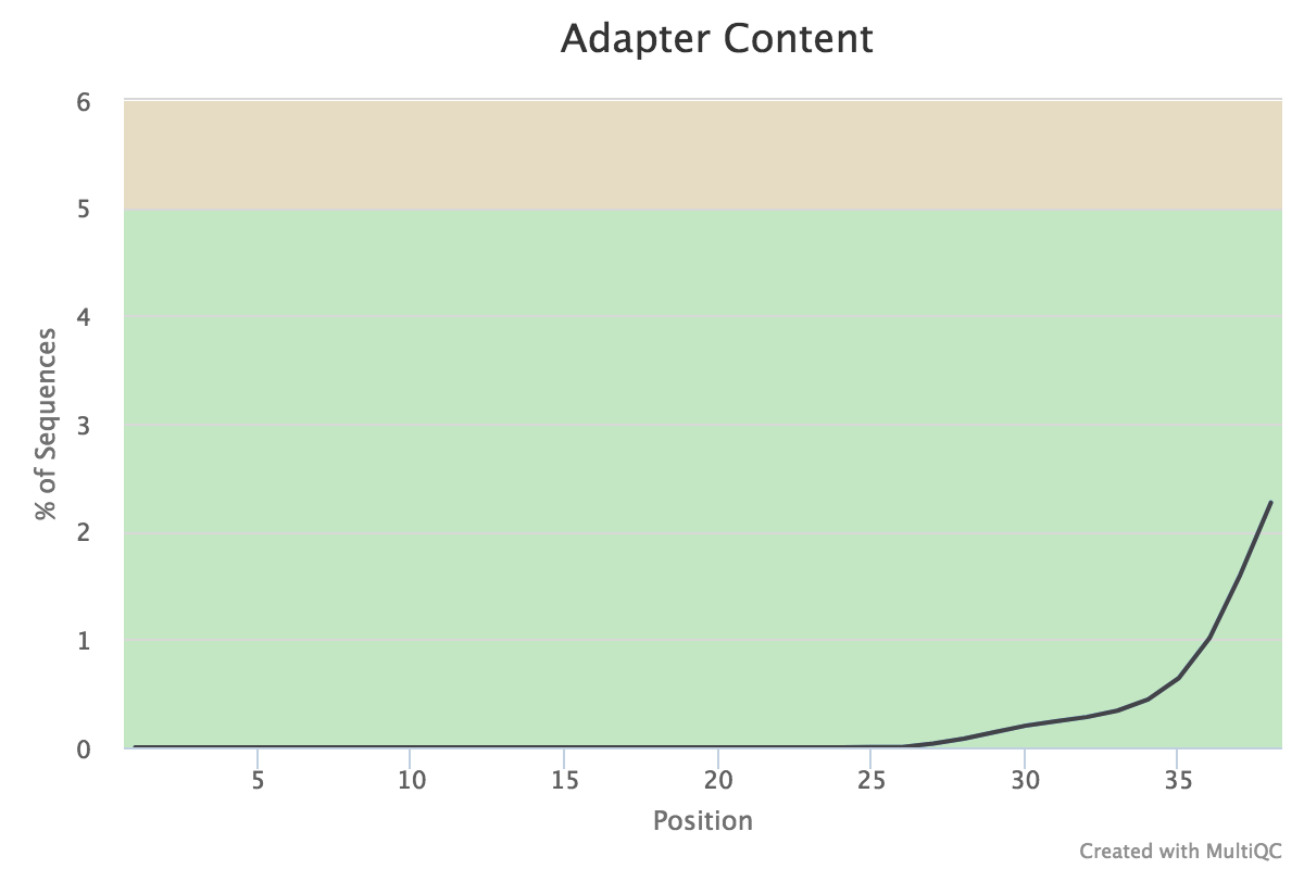
However, if transposase adapters were present in large amounts the raw reads, we can remove them using one of many adapter trimming programs, for example cutadapt.
3. Download Arabidopsis Genome
Before starting the alignment, we need the Arabidopsis genome, which one can download from either Araport or EnsemblPlants.
We already have the Arabidopsis genome downloaded, so we make a symbolic link or shortcut to it and then refer to the link for the making the index.
1
ln -s /path/to/Arabidopsis_thaliana.TAIR10.dna.toplevel.fa At_Genome
The shortcut we have made is At_Genome
We will use bowtie2 to align and the following sections describe the making of the index and the alignment.
4. Building the bowtie2 Genome Index
We use environment modules in our cluster, so load the appropriate module and get going.
1
2
3
module load bowtie2
mkdir bwt_index
bowtie2-build At_Genome bwt_index/At.TAIR10
5. Alignment using bowtie2
1
bowtie2 --threads 8 -x bwt_index/At.TAIR10 -q -1 ATAC_paired/SRR4733912_1.fastq.gz -2 ATAC_paired/SRR4733912_2.fastq.gz -S bwt_out/SRR4733912.sam
a) Convert SAM to BAM and sort
1
 samtools view --threads 7 -bS SRR4733912.sam | samtools sort --threads 7 - > SRR4733912.sorted.bam
View the header of the sorted BAM file:
1
2
3
4
5
6
7
8
9
10
samtools view -H SRR4733912.sorted.bam
 @HD     VN:1.0  SO:coordinate
 @SQ     SN:1    LN:30427671
 @SQ     SN:2    LN:19698289
 @SQ     SN:3    LN:23459830
 @SQ     SN:4    LN:18585056
 @SQ     SN:5    LN:26975502
 @SQ     SN:Mt   LN:366924
 @SQ     SN:Pt   LN:154478
 @PG     ID:bowtie2      PN:bowtie2      VN:2.2.6        CL:"/opt/rit/app/bowtie2/2.2.6/bin/bowtie2-align-s --wrapper basic-0 --threads 8 -x bwt_index/At.TAIR10 -q -S bwt_out/SRR4733912.sam -1 /tmp/26409.inpipe1 -2 /tmp/26409.inpipe2"
b) Index the BAM file
1
 samtools index SRR4733912.sorted.bam
the index file is SRR4733912.sorted.bam.bai
It is important to identify and remove reads aligning to Mt and Chloroplast in case of ATAC-seq because this can cause confounding signals.
1
 samtools idxstats SRR4733912.sorted.bam | cut -f1 | grep -v Mt | grep -v Pt | xargs samtools view --threads 7 -b SRR4733912.sorted.bam > SRR4733912.sorted.noorg.bam
We call the BAM file without chloroplastic and mitochondrial alignments as SRR4733912.sorted.noorg.bam
One can compare the index stats of the BAM file without organellar DNA alignments and the file with all alignments. You can use this to bench mark the alignment and the procedure used to make the libraries.
1
2
3
4
5
6
7
8
9
10
11
12
13
14
15
16
17
18
19
20
 samtools idxstats SRR4733912.sorted.noorg.bam
 1       30427671        2018268 43655
 2       19698289        2796545 47708
 3       23459830        1738071 36100
 4       18585056        1290746 26515
 5       26975502        1795689 40246
 Mt      366924  0       0
 Pt      154478  0       0
 *       0       0       3016596
########################################################

 samtools idxstats SRR4733912.sorted.bam
 1       30427671        2018268 43655
 2       19698289        2796545 47708
 3       23459830        1738071 36100
 4       18585056        1290746 26515
 5       26975502        1795689 40246
 Mt      366924  2469591 35167
 Pt      154478  44476436        524929
 *       0       0       3016596
6) PEAK Calling
We can now call the peaks/pileups of reads in our sample. We use macs2 for that. However there are other peak calleing algorithm as well, check this for a good review. macs2 was designed originally for CHIPseq but works just as well for ATAC-seq.
1
  macs2 callpeak -t /path/to/SRR4733912.sorted.noorg.bam -q 0.05 --broad -f BAMPE -n SRR4733912 -B --trackline --outdir . &>SRR4733912.peak.log&
Important Parameters used:
1
2
3
4
5
6
7
8
9
10
11
12
13
14
15
16
17
 Used a local lambda for noise reduction in the vicinity of peaks.
 # ARGUMENTS LIST:
 # name = SRR4733912
 # format = BAMPE
 # ChIP-seq file = ['../bwt_out/SRR4733912.sorted.noorg.bam']
 # control file = None
 # effective genome size = 2.70e+09
 # band width = 300
 # model fold = [5, 50]
 # qvalue cutoff for narrow/strong regions = 5.00e-02
 # qvalue cutoff for broad/weak regions = 1.00e-01
 # Larger dataset will be scaled towards smaller dataset.
 # Range for calculating regional lambda is: 10000 bps
 # Broad region calling is on
 # Paired-End mode is on
 # mean fragment size is determined as 139 bp from treatment
 # fragments after filtering in treatment: 4002590
The following files will be output:
1
2
3
4
5
SRR4733912_control_lambda.bdg
SRR4733912_peaks.broadPeak
SRR4733912_peaks.gappedPeak
SRR4733912_peaks.xls
SRR4733912_treat_pileup.bdg
We have the treatment pileup bedgraph file SRR4733912_treat_pileup.bdg, which we can convert to a bigwig format to view in a browser, e.g., IGV. We download a few program available from UCSC(https://genome.ucsc.edu/); bedClip and bedGraphToBigWig. We will also make use of bedtools.
a) Make a chromsome sizes file
1
bioawk -c fastx '{print $name, length($seq)}' /path/At_Genome > At_chr.sizes
b) Clip the bed graph files to correct coordinates
1
 bedtools slop -i SRR4733912_treat_pileup.bdg -g At_chr.sizes -b 0 | /path/to/bedClip stdin At_chr.sizes SRR4733912_treat_pileup.clipped.bdg
c) Sort the clipped files
1
 sort -k1,1 -k2,2n SRR4733912_treat_pileup.clipped.bdg > SRR4733912_treat_pileup.clipped.sorted.bdg
d) Convert to bigwig
1
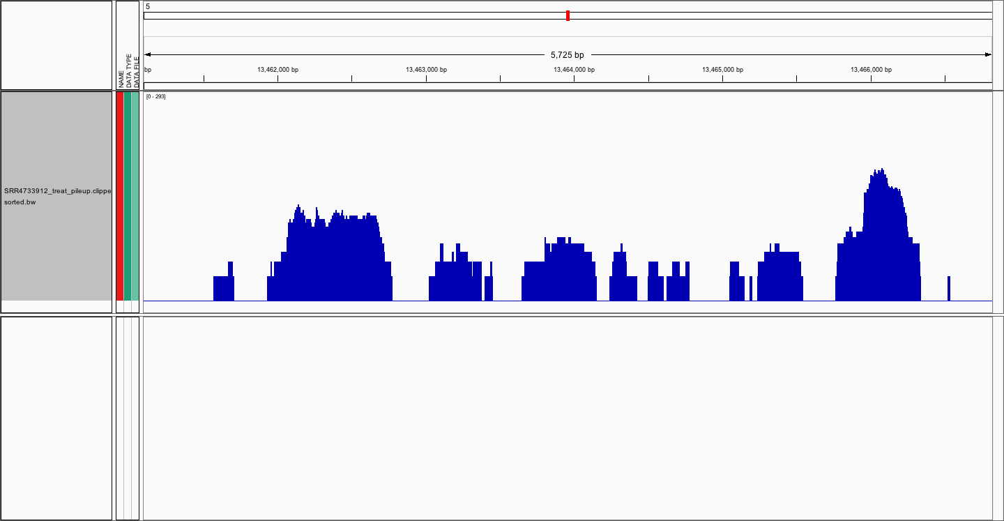
/path/to/bedGraphToBigWig SRR4733912_treat_pileup.clipped.sorted.bdg At_chr.sizes SRR4733912_treat_pileup.clipped.sorted.bw
We can now directly view the bigwig file in the IGV Genome browser or calculate peak scores over a genomic region/interval using UCSC’s bigwigaverageoverbed.